




TL;DR: Seasonal trading takes a position because of the date, so the real decision is whether a calendar window is an edge or a coincidence. On 20 years of six futures markets, 8 of 72 month cells pass a t-test, about what shuffled calendars produce. Unadjusted continuous futures data can invent seasonal patterns at contract rolls, so clean the data first. Size any seasonal window from its worst adverse excursion, not its average return.
Seasonal trading sounds like the easiest edge in the market. Natural gas meets cold weather every winter, corn gets harvested every autumn, and stock indices have their famous "good months". If the calendar repeats, why not trade the calendar?
The catch is that 20 years of history gives you only 20 Julys. That is a small sample, and small samples are very good at producing confident-looking averages out of noise. This guide explains what seasonal trading is, why seasonal patterns can exist, and then tests the idea on a 20-year calendar of six futures markets so you can see which patterns hold up, which ones were never real, and what it takes to size a seasonal trade without letting one bad year end it.
What Seasonal Trading Means
Seasonal trading means taking a position because a market has historically leaned one way during a specific calendar window, rather than because of what the chart is doing right now. A seasonal trader might buy in a particular month, sell a particular contract ahead of a weather season, or hold a spread between two delivery months that tends to move at the same time each year.
The claim underneath every seasonal trade is narrow. It says that over a long sample, a market has leaned in one direction during a stated window, and that a mechanism behind that lean could repeat next year.
The three ingredients of a tradeable seasonal pattern
A seasonal window is only worth trading when three things line up.
- A stated window, with the entry and exit rule written down before you look at the results.
- A sample large enough to separate an edge from luck, which is usually far larger than traders expect.
- A mechanism, meaning some reason the flow should exist again next year, such as a heating season, a harvest, a tax deadline or a regular index flow.
Miss one of the three and you are not trading a seasonal pattern. You are trading a memory of a chart.
Seasonal trading also differs from trend or pattern trading in what it ignores. A breakout trader reacts to price. A seasonal trader commits to a window in advance and accepts that the current chart may disagree. That is both the appeal (a plan made away from the noise of the moment) and the risk (the window can be wrong for the whole month while you sit in it).
Why Seasonal Price Patterns Happen
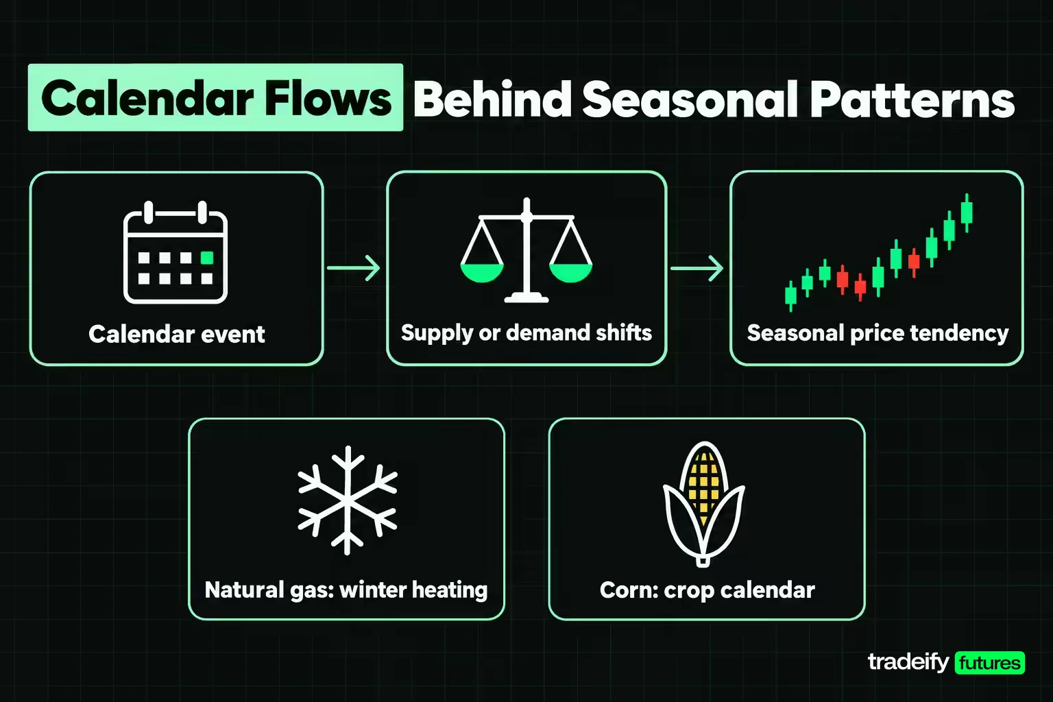
Seasonal price patterns, where they are real, come from flows that are tied to the calendar, and that is where seasonal trading has its strongest footing. The clearest examples are in commodities, where weather and the growing cycle change supply or demand on a schedule.
- Natural gas and the heating season. The U.S. Energy Information Administration (EIA) says U.S. natural gas consumption typically peaks during the winter heating season, November to March, when colder temperatures raise space-heating demand in homes and commercial buildings. A seasonal trader sees that and expects winter contracts to carry a premium, and expects prices to react sharply when early-winter weather turns out milder or colder than the market priced.
- Corn and the crop calendar. The USDA's National Agricultural Statistics Service lists the most active corn planting dates in Iowa as April 25 to May 18 and the most active harvest dates as October 5 to November 9. In Illinois, planting is most active April 21 to May 23 and harvest September 23 to November 5. Uncertainty about the size of a crop is highest while it is growing, and supply arrives in a rush at harvest, so the calendar shapes both risk and price.
- Crude oil and the driving season. The EIA defines the summer driving season for gasoline and diesel as April through September. Refiners build product ahead of that demand, which can change crude demand in the months before and during the season.
- Gold. Gold is often said to have seasonal physical demand around year-end festivals and gift-buying in Asia. That explanation is widely repeated, but the calendar study in this guide cannot confirm it, so treat it as a hypothesis rather than a mechanism you can count on.
Why a known seasonal flow does not guarantee a seasonal price move
Here is the part most seasonal content skips. A flow that everyone knows about is usually already in the price. If every trader knows winter heating demand is coming, the futures curve already charges more for January gas than for May gas. The price move that a seasonal trader actually earns comes from the gap between what the market expected and what happened, which is why a known mechanism is necessary but not sufficient.
That is also why a seasonal average with no mechanism behind it deserves suspicion. If you cannot name the flow, the most likely explanation for a strong average is chance.
Behavioral Factors Behind Seasonal Stock Patterns
For seasonal trading in stock indices, the drivers are less physical than corn or natural gas, so the explanations lean on behavior, cash flows and incentives. These are the ones most often proposed for seasonal stock patterns.
- Payment flows at the turn of the month. Salaries, pension contributions and fund inflows tend to arrive around month-end. Robert Ariel's 1987 study in the Journal of Financial Economics found that, over 1963 to 1981, mean stock returns were positive only for days immediately before and during the first half of calendar months.
- Tax-loss selling. Investors who sell losing positions before year-end to realize tax losses can push those stocks down in December, with a rebound often expected in January. This is the usual explanation offered for the January effect.
- Window dressing. Some fund managers are said to buy recent winners and dump losers before quarter-end reports, which can move prices around reporting dates.
- Mood and attention. Holiday periods, summer vacations and lower volume are often cited for weaker or quieter stretches, and for the "Santa Claus rally" around the end of December.
Why behavioral seasonal effects fade
Behavioral explanations have a weakness that physical ones do not. Once a seasonal effect is published and traders act on it, they buy earlier and earlier to get ahead of each other, and the effect can shrink or move. Corn still gets harvested in autumn no matter how many people know about it. A turn-of-month effect has no such anchor. That is a good reason to give behavioral seasonal patterns a shorter leash and to recheck them on recent data, not only the full history.
How Economic Cycles Distort Seasonal Trading Patterns
Seasonal trading windows sit on top of other calendars that are also predictable, and those overlaps can produce or hide a seasonal pattern.
- Earnings seasons. Most large U.S. companies report in the weeks after each quarter ends. A strong July average in stock indices, for example, overlaps with second-quarter earnings, so a "July effect" may really be an earnings-season effect that would move if reporting habits changed.
- The tax calendar. Year-end tax decisions and early-year contributions to retirement accounts change flows around December, January and April.
- Elections. Election years change policy uncertainty, and some traders track a four-year presidential cycle. With only a handful of cycles in any modern sample, that is the clearest example of a pattern with far too few observations to test properly.
- Central bank meetings and data releases. Scheduled releases (inflation, employment, central bank decisions) fall at fixed points in the month. A seasonal window that contains a major release is partly a bet on that release.
- The business cycle. Recessions and recoveries do not follow the calendar, but they dominate a 20-year sample. One crisis year in a 20-observation cell can decide the average on its own.
Sector rotation and seasonal trading
Sector rotation is the stock-market version of the overlap between seasonal trading windows and the economic cycle. Energy demand, retail spending and travel all have seasonal peaks, and some traders rotate between sectors to follow them. The same discipline applies. A sector's seasonal tilt needs a mechanism, a stated window and enough years before it becomes a rule, and the sector's own performance in the wider economic cycle can swamp the calendar effect.
How the 20-Year Seasonal Futures Calendar Was Built
To see what seasonal trading looks like in real futures data, this guide uses a simple, repeatable study. The method is stated in full so you can repeat it or attack it.
- Markets. Six futures markets with different drivers: the E-mini S&P 500 (ES), E-mini Nasdaq-100 (NQ), gold (GC), WTI crude oil (CL), Henry Hub natural gas (NG) and corn (ZC).
- Data. Daily closes of each market's front continuous futures series from Yahoo Finance, read on November 4, 2026.
- Sample. November 2006 to October 2026, which is 240 months and exactly 20 observations of each calendar month in each market, for 72 market-month cells.
- Return. A month's return is its last close divided by the previous month's last close, minus one. That entry price is knowable and tradeable before the month starts.
- Roll adjustment. A continuous futures series switches from the expiring contract to the next one on a roll session. Using each contract's last trading day under CME rules, the first session after every expiry is dropped from the return. That removes 83 roll sessions from ES, 83 from NQ, 125 from gold, 251 from crude oil, 251 from natural gas and 104 from corn.
- Adverse excursion. For each window, the lowest close inside the month relative to the entry close (the highest close for a short window). It uses closing prices only, so a real intraday excursion would be worse.
- Statistics. For each cell, the mean, median, number of years higher, a one-sample t-statistic, and a split-half check comparing the first ten years with the last ten.
What the roll adjustment costs
Dropping one session per contract roll, as the 20-year seasonal futures calendar study does, is a blunt fix. It removes the contract switch, but it also removes that session's genuine price move. For quarterly equity index contracts that is four sessions a year and changes little. For monthly contracts like crude oil and natural gas it is twelve sessions a year, so treat their grid values as rougher than the equity index values. The alternative, using the unadjusted continuous series, is far worse, because contract switches land in the same months every year and show up as fake seasonal moves.
Related lesson: Continuous futures contracts
Roll Gaps That Fake Seasonal Patterns in Futures

Roll gaps are the biggest data trap in futures seasonal trading. A continuous futures series is a chain of separate contracts. When the front contract expires, the series jumps to the next delivery month, and the price difference between the two contracts appears as a one-day "move" that no trader ever experienced. Because contracts expire on a fixed schedule, those jumps land in the same calendar months every year, which is exactly what a seasonal screen is looking for.
Corn is the cleanest example. Corn futures trade for March, May, July, September and December delivery, and each contract stops trading on the business day before the 15th of its delivery month. The July contract prices old-crop corn still in storage, while the September contract is priced closer to the coming harvest. In tight years that gap is large. On the unadjusted continuous series, the session after the July contract expired showed a close-to-close drop of 17.39% in 2021, 13.06% in 2022 and 16.76% in 2023. None of those were price moves a corn holder lived through. They were contract switches.
Roll-adjusted versus unadjusted seasonal cells
The table compares five seasonal cells from this guide's 20-year study (Yahoo Finance daily closes) on the unadjusted continuous series with the same cells after the roll session is removed.
| Market and month | Unadjusted continuous series | Roll session removed | Years up, unadjusted | Years up, roll removed |
|---|---|---|---|---|
| Corn (ZC) Dec | 5.72% | 3.31% | 18 of 20 | 13 of 20 |
| Corn (ZC) Jul | -5.19% | -1.31% | 6 of 20 | 8 of 20 |
| Natural gas (NG) Sep | 7.63% | 2.08% | 13 of 20 | 9 of 20 |
| Natural gas (NG) Apr | 5.31% | 2.15% | 16 of 20 | 12 of 20 |
| Natural gas (NG) Dec | -9.13% | -7.79% | 7 of 20 | 5 of 20 |
Corn in December looks like one of the most reliable seasonal trades in futures on the raw series, up in 18 of 20 years. Remove the roll and it is up in 13 of 20, with the average cut by more than two points. Natural gas in September drops from 7.63% to 2.08%. Natural gas in April falls from 16 winning years to 12.
The practical rule is simple. Before you trust any futures seasonal chart, find out whether it is built from an unadjusted continuous series, a back-adjusted series, or individual contracts. If the tool does not say, check the pattern against single contract months yourself.
Related lesson: Futures rollover
The 20-Year Futures Seasonal Calendar by Month
The 20-year futures seasonal calendar shows the roll-adjusted mean monthly return for each market and month from November 2006 to October 2026. Read it as a map of where the averages sit, not as a trade list. Each cell is the average of only 20 months.
| Market | Jan | Feb | Mar | Apr | May | Jun |
|---|---|---|---|---|---|---|
| E-mini S&P 500 (ES) | 0.06% | -0.04% | 0.70% | 2.29% | 0.99% | 0.38% |
| E-mini Nasdaq-100 (NQ) | 0.71% | 0.32% | 0.95% | 2.86% | 2.36% | 0.84% |
| Gold (GC) | 3.42% | 1.29% | 0.06% | 0.83% | -0.14% | -1.47% |
| WTI crude oil (CL) | -0.36% | 3.82% | 2.27% | 1.24% | 2.68% | 3.15% |
| Natural gas (NG) | 7.72% | -4.82% | -1.30% | 2.15% | 1.54% | 1.19% |
| Corn (ZC) | 1.12% | 0.96% | -0.12% | 2.73% | -0.89% | -2.11% |
| Market | Jul | Aug | Sep | Oct | Nov | Dec |
|---|---|---|---|---|---|---|
| E-mini S&P 500 (ES) | 2.38% | 0.18% | -0.03% | 0.72% | 2.15% | 0.71% |
| E-mini Nasdaq-100 (NQ) | 3.26% | 0.87% | -0.04% | 0.91% | 1.77% | 0.30% |
| Gold (GC) | 1.26% | 2.11% | -0.27% | -0.04% | 1.01% | 0.55% |
| WTI crude oil (CL) | 1.43% | -2.27% | 0.50% | 0.99% | -3.92% | -0.99% |
| Natural gas (NG) | -4.16% | -0.61% | 2.08% | -2.36% | 1.05% | -7.79% |
| Corn (ZC) | -1.31% | 0.15% | -1.42% | 1.88% | -0.84% | 3.31% |
Reading the seasonal grid for drift and volatility
Three things stand out before any statistics.
First, most stock-index cells are positive because the indices rose over the period. The average ES month was 0.87% and the average NQ month was 1.26%, so a positive month for those markets proves little on its own. The useful question is whether a month beats its market's normal month.
Second, the energy markets own the extremes. Natural gas January averages 7.72%, but that cell's t-statistic is only 0.98, because two explosive years carry it. Natural gas has a monthly standard deviation of 17.12% across the sample, against 4.33% for ES. A big number in a volatile market is mostly volatility.
Third, the cells that look like stories (gold in January, Nasdaq in July, natural gas weak in December) need a test before they become a plan. That test is the job of a significance screen.
Which Seasonal Cells Survive a Significance Test
Screening for seasonal trading setups means testing every cell of a seasonal calendar at once, and that creates a problem. If you test 72 cells, some will look significant by luck.
Using a t-statistic of 2.0 as the screen, 8 of the 72 cells pass. A t-statistic of 2.0 with 19 degrees of freedom has a two-sided p-value of 0.0600, so about 4.32 cells would pass by chance even if the calendar meant nothing. Eight sounds better than four, but that simple chance estimate assumes returns behave nicely, and market returns do not.
A tougher check shuffles the history. Keeping each market's 240 monthly returns but randomly reassigning which month each one belongs to, 2,000 times, shuffled calendars flag 7.73 cells on average, and 53% of them flag 8 or more. In other words, the real calendar produced about as many "significant" seasonal cells as a random calendar built from the same markets. Upward drift and fat tails alone can produce that many.
Multiple testing points the same way. The Bonferroni threshold for 72 tests at the 5% level with 19 degrees of freedom is a t-statistic of 4.04. The strongest cell in the grid, NQ in July, has a t-statistic of 3.43 and a nominal p-value of 0.0028. Adjusted for 72 tests, that p-value becomes 0.20. No single cell would survive as a standalone discovery.
The seasonal cells that passed the first screen
| Market and month | Mean | Years up | t-statistic | First 10 years | Last 10 years | Median adverse excursion | Worst adverse excursion |
|---|---|---|---|---|---|---|---|
| E-mini Nasdaq-100 (NQ) Jul | 3.26% | 17 of 20 | 3.43 | 3.73% | 2.79% | -0.74% | -10.42% |
| Gold (GC) Jan | 3.42% | 14 of 20 | 3.33 | 3.74% | 3.10% | 0.12% | -8.70% |
| E-mini S&P 500 (ES) Jul | 2.38% | 15 of 20 | 3.21 | 1.87% | 2.88% | -1.03% | -5.43% |
| WTI crude oil (CL) Feb | 3.82% | 15 of 20 | 2.50 | 5.13% | 2.50% | -3.29% | -22.04% |
| Natural gas (NG) Dec | -7.79% | 5 of 20 | -2.35 | -5.42% | -10.17% | -2.11% | -23.56% |
| Corn (ZC) Dec | 3.31% | 13 of 20 | 2.34 | 4.46% | 2.17% | -1.70% | -16.02% |
| E-mini S&P 500 (ES) Nov | 2.15% | 14 of 20 | 2.31 | 0.17% | 4.13% | -0.87% | -22.64% |
| E-mini S&P 500 (ES) Apr | 2.29% | 16 of 20 | 2.09 | 2.58% | 2.00% | -1.42% | -11.20% |
Natural gas December is a short window, so its adverse excursion measures the highest close above entry, shown as a negative number like the others. A positive median adverse excursion, as for gold in January, means the median year never closed below the entry price.
What the split-half check adds
In the 20-year futures seasonal calendar, persistence is the one piece of evidence that favors the 8 cells that passed a t-statistic of 2.0. Across all 72 cells, only 38 keep the same sign in the first ten years and the last ten. All 8 flagged cells do. That is worth something, but read the halves before you read the average. E-mini S&P 500 November averaged 0.17% in the first ten years and 4.13% in the last ten. That is a pattern that arrived late, not one that persisted, and a late arrival is exactly what a shifting regime looks like.
The honest reading is that the grid is suggestive, not proof. That is less exciting than a list of "best months", and more useful. A handful of seasonal cells have consistent direction and a plausible story, and none of them is strong enough to trade on the calendar alone.
How Much of a Seasonal Window Comes From a Few Sessions
A monthly average hides the path through the month. To see where a seasonal return actually comes from, each month in the calendar study was rebuilt from its daily returns with the two best sessions removed. This is a concentration test, not a trading rule. It asks a simple question: if you had missed the two best days of every window, would the window still have paid?
The answer is no, almost everywhere. Across all 72 cells, the average month is 0.57%, and with the two best sessions removed it becomes -4.97%. Before the strip, 49 cells are positive. After it, none are. For the 8 flagged cells, the average falls from 1.60% to -3.37%. Nasdaq in July drops from 3.26% to -0.49%, gold in January from 3.42% to -0.39%, and the S&P 500 in July from 2.38% to -0.52%.
That result is less damning than it looks, because removing the two best days hurts any month in any market. The fairer comparison is against the market's own normal month, with the same two days stripped from both. On that basis the 8 flagged seasonal cells keep their edge in 8 of 8 cases, by an average of 2.80 percentage points a month, or 2.77 points once the two best sessions are removed from both the window and the baseline. Nasdaq in July beats an ordinary Nasdaq month by 2.00 points (2.33 stripped), gold in January by 2.70 points (2.36 stripped) and the S&P 500 in July by 1.50 points (1.96 stripped).
So two things are true at once. The excess over normal drift is the more durable part of a seasonal window. And the money in any single window still arrives in a few sessions you cannot schedule, which means execution and staying power decide whether you collect it.
How Many Years of Data Seasonal Analysis Needs
Seasonal trading research needs far more history than most traders use, because every year adds only one observation per month. A 10-year chart of "how July behaves" is a sample of 10.
A standard power calculation shows the scale of the problem. Take a monthly return standard deviation of 3.31%, which is what E-mini S&P 500 July showed in the study. To have an 80% chance of detecting a real edge at the usual 5% significance level, you need about:
- 24 years of data for a 2.0% monthly edge
- 88 years for a 1.0% edge
- 346 years for a 0.5% edge
Using ES's all-month standard deviation of 4.33% instead, a 2.0% edge needs 39 years and a 1.0% edge needs 149. No futures market has that much clean history. That is why seasonal research on five or ten years of data mostly produces confident statements about noise.
Seasonal data sources and their weaknesses
- Continuous futures series. Free and easy, but often unadjusted, so check for roll gaps before trusting any seasonal pattern built on them.
- Individual contract history. The cleanest data for seasonal trading in futures, especially for seasonal spreads, but harder to collect for expired contracts.
- Cash or ETF proxies. An index or a fund that holds the underlying can give a longer history without roll gaps, at the cost of measuring something slightly different from the futures contract.
- Fundamental calendars. The EIA, USDA and central banks publish the schedules that create seasonal flows. They are the mechanism check, not the price data.
A useful habit is to note the start date of every seasonal chart you look at. A pattern that only appears when the sample starts in a particular year is a pattern about that starting year.
Seasonal Trading Strategies With Entry and Exit Rules
Seasonal trading strategies come in three common forms, and each needs an entry rule, an exit rule and an invalidation written before the window opens.
- Calendar window. Enter at a fixed point (for example, the last close before the month) and exit at a fixed point (the month's last close). This is what the calendar study measures.
- Seasonal spread. Buy one delivery month and sell another in the same market, such as an old-crop and new-crop grain spread, to trade the seasonal relationship between them rather than outright direction.
- Seasonal filter. Use the seasonal tilt only to choose direction, then take entries from your normal setup inside the window. The calendar decides which side you look for. The chart decides whether there is a trade.
The ES July seasonal window in a strong year
Take the cleanest equity window in this guide's 20-year futures study (Yahoo Finance daily closes), E-mini S&P 500 July, which was up in 15 of 20 years with a median of 2.04%. ES is worth $50 per index point.
In 2022, the June 30 close was 3,789.50 and the July 29 close was 4,133.50. That is a gain of 344.00 points, or $17,200 per contract, a 9.08% month. The lowest close inside the window, 3,793.25, was still above the entry, so the trade never showed a closing loss. It is the kind of month that makes a seasonal rule look obvious in hindsight.
The ES July seasonal window in a losing year
The same E-mini S&P 500 July window, at $50 per index point, went the other way in 2026. The June 30 close was 7,548.25 and the July 31 close was 7,519.25. That is a loss of 29.00 points, or $1,450 per contract, only -0.38% on the month. The path was worse than the result. The lowest close inside the window was 7,351.25, which is 197.00 points below entry, or $9,850 per contract and -2.61%. At entry, one contract controlled about $377,412.50 of index exposure.
Compared with the strong 2022 window, this was the same month, same rule and same instrument. The losing year looks harmless on the final number. It still asked whoever held it to sit through a drawdown almost seven times the size of the final loss, and that is the moment when most people abandon the plan.
What stop distance does to a seasonal window
Seasonal trading windows are not precise enough for tight stops. Using closing prices only, a 2% stop on ES July was touched in 6 of 20 years and cut the average result from 2.38% to 1.69%. A 5% stop was touched once, in 2008, and the average became 2.18%. For NQ in July, a 2% stop was touched in 5 of 20 years and the average became 2.71%. For gold in January, a 2% stop was touched in 6 of 20 years and the average was 3.02%.
The trade-off is plain. A seasonal edge, if it exists, is spread across the whole window, not delivered on day one. A stop tight enough to feel comfortable will often take you out before the window does its work, and a stop wide enough to survive the window demands a much smaller position. That is a sizing question, not a stop-placement question.
Sizing a Seasonal Trade From the Adverse Excursion
In seasonal trading, the average return tells you whether a window might be worth taking. The adverse excursion tells you whether you can afford it. Size from the second number.
- Record the window's median and worst adverse excursion over a long sample, on closing prices.
- Decide the share of equity one window may draw down. One percent is a common starting point.
- Convert that allowance to dollars and divide by the adverse excursion in dollars for one contract.
- Check the answer against the worst excursion. If the worst case breaks your limit at one contract, the trade does not fit that account at that size.
Worked sizing example for a seasonal window
Use an illustrative ES price of 6,000. One ES contract controls 6,000 x $50 = $300,000. E-mini S&P 500 July has a median adverse excursion of 1.03% and a worst of 5.43%, so one contract would expect a median drawdown of about $3,090 and a worst case of about $16,290.
On $50,000 of equity with a 1% allowance, the budget is $500. That supports 0.16 contracts on the median excursion and 0.03 contracts on the worst. In other words, one full ES contract does not fit.
The Micro E-mini S&P 500 (MES) is worth $5 per point, one tenth of ES. At the same illustrative 6,000, one MES controls $30,000, with a median excursion of about $309 and a worst case of about $1,629. The $500 budget covers 1.62 contracts on the median and 0.31 on the worst. One micro fits the median case. The worst case still breaks the budget, which is the decision a seasonal trader has to make before the month starts, not during it.
Natural gas in December shows the problem at its sharpest. As a short window it averaged -7.79%, a strong result for a short, but its worst adverse excursion was 23.56%. Using closing prices, a 2% stop on that short was touched in 10 of 20 years. Being right about direction on average is not the same as being able to hold the position through the bad years.
Related lesson: Volatility-based position sizing
Seasonality Tools for Finding Seasonal Trading Patterns
Seasonality tools turn price history into seasonal charts and screens for seasonal trading ideas. They save time, but each one makes choices about data and method that you need to know before you trust the output.
- Seasonal chart features in charting platforms. TradingView's Seasonals tool, for example, plots price change over the same period in different years on one chart and can add an average line across the selected years. That makes it easy to see whether a pattern is consistent or carried by one or two years.
- Dedicated seasonal screeners. Commercial seasonal services scan many markets for windows with high historical hit rates. Check how many windows they test, because a screener that tests thousands of start and end dates will always find impressive ones by chance.
- Spreadsheets and scripts. A spreadsheet or a short Python script can build your own seasonal grid from daily closes. This is the only route where you control the roll handling, the sample start and the statistics.
- Fundamental calendars and reports. EIA reports on natural gas and petroleum, USDA crop calendars and crop progress data, and central bank meeting schedules tell you whether a seasonal mechanism is present this year.
Checklist for judging a seasonality tool
- How the futures history is built (unadjusted continuous, back-adjusted or individual contracts).
- The sample start and end dates, and whether incomplete months are dropped.
- Whether it reports the number of years higher, the median and the spread, not only the average.
- Whether it shows how many windows were searched to find the one it highlights.
- Whether it shows adverse excursion or drawdown inside the window.
A tool that shows only "up in 15 of the last 20 years" has told you the least useful thing about a seasonal pattern.
How to Backtest a Seasonal Trading Pattern
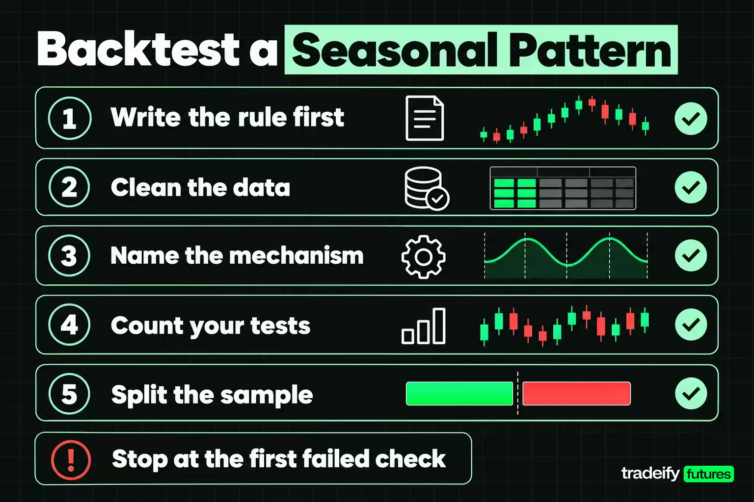
Backtesting a seasonal trading pattern follows the same logic as any strategy test, with extra care for small samples. Run these checks in order and stop as soon as one fails.
- Write the rule first. State the market, the window, the entry and exit convention and the direction before you look at returns. Count the observations. Under about 15, a large apparent edge is usually an artifact.
- Clean the data. Remove or adjust contract rolls, drop incomplete months and record the exact sample dates.
- Name the mechanism. If you cannot name the flow that creates the seasonal tendency, expect it to decay.
- Count your tests. If you searched many windows or markets, compare your best result with what a shuffled calendar produces.
- Split the sample. If the first half and the second half disagree on direction, you are looking at a regime, not a season.
- Strip the best sessions. Remove the two best days from every window and compare the window with the market's own normal month on the same basis.
- Measure the path. Record the median and worst adverse excursion and check them against your sizing limits.
- Subtract costs. Commissions, slippage on entry and exit, and, for futures, the cost of rolling if the window crosses an expiry.
Metrics worth recording for a seasonal backtest
- Mean and median return, and the number of years higher
- t-statistic and how many windows were tested to find this one
- First-half and second-half averages
- Excess over the market's normal month
- Median and worst adverse excursion
- Result with realistic stops and costs
Keep a journal of each live seasonal window as well: the entry and exit, the worst point, and whether the mechanism actually showed up that year. With so few observations, every new year matters.
Related lesson: Backtesting a trading strategy
Famous Seasonal Stock Market Patterns Put to the Test
The most quoted seasonal patterns come from stocks. Several of them can be checked on the same kind of data used for the futures calendar, and they are weaker than their reputation.
Sell in May and the Halloween effect
"Sell in May and go away" says stocks do better from November to April than from May to October. Bouman and Jacobsen's 2002 paper in the American Economic Review, "The Halloween Indicator", made it a famous academic puzzle.
In this guide's calculation on SPY total-return data from Yahoo Finance, across 33 seasons from November 1993 to October 2026, the November to April half averaged 7.28% and the May to October half averaged 4.21%. Both halves were positive in 26 of 33 seasons. A paired t-test gives a t-statistic of 1.44 and a p-value of 0.16, so the difference is not statistically distinguishable from noise. Over the last 15 seasons the halves came in at 7.74% and 7.07%, with a p-value of 0.81. Selling in May would have meant giving up a positive summer return in most years.
The turn-of-the-month effect
The turn-of-the-month effect says returns concentrate in the last session of a month and the first three of the next. Across the six futures markets from November 2006 to October 2026, pooled and roll-adjusted, those 5,754 sessions averaged 0.0306% each, against 0.0269% for the other 24,428 sessions. That is a difference too small to trade after costs.
The weakest months for stocks on the SPY record
On the same SPY record, September was the weakest month at -0.47% on average, higher in only 18 of 34 years, but with a t-statistic of -0.56. February averaged -0.03% and August 0.06%. These are soft months, not reliable shorts. The strongest months were November at 2.45% with a t-statistic of 3.35, April at 2.00% (t 2.52) and July at 1.42% (t 2.19). January, home of the famous January effect, averaged 0.76% with a t-statistic of 1.06, and December, home of the Santa Claus rally, averaged 0.97% with a t-statistic of 1.63.
The lesson for seasonal trading is the same across all of these. A seasonal story with a real tilt in a long sample can still be too weak, too late or too costly to trade on its own.
Seasonal Trading on an Intraday Funded Account
Seasonal trading and intraday funded-account rules pull in different directions. A seasonal window lasts weeks, while many prop-firm accounts require every position to be flat each day. That leaves two honest ways to use seasonal research inside intraday rules: as a directional bias that decides which side of the market you look for setups on, and as a risk flag that tells you when a market is entering a historically volatile stretch, such as natural gas in early winter.
A seasonal bias is not a setup. If the window says long and the session gives you no valid long entry, there is no trade, and forcing one because "July is usually up" is the same mistake as chasing a missed breakout. Seasonal research also says nothing about the next hour, so intraday stops and daily loss limits still do the risk work.
On our accounts, every position must be closed by 4:45 PM ET and there are no overnight, weekend or swing holds, so a month-long seasonal window cannot be held as one position. Our hedging rule also prohibits opposing positions on the same instrument or on two products in the same Product Group, which means a long-and-short seasonal spread between two delivery months of the same market is not something you can run on our accounts. What fits is using the seasonal tilt on supported markets such as ES, NQ, GC, CL, NG or ZC to choose the side of your intraday trades.
Seasonal Trading FAQ
What is seasonal trading?
Seasonal trading is taking a position because a market has historically leaned one way during a specific calendar window. A tradeable seasonal pattern needs a stated window, a large enough sample and a mechanism, such as a heating season or a harvest, that could make it repeat.
Is seasonal trading reliable?
Only partly. In this guide's 20-year study of six futures markets using Yahoo Finance daily closes, 8 of 72 month cells passed a t-test, about as many as shuffled calendars produced, and none survived a correction for testing 72 cells. The flagged cells did beat their market's normal month in 8 of 8 cases, so a seasonal tilt can inform a bias but is weak as a standalone rule.
What are the two worst months for stocks to buy?
In this guide's calculation on SPY total-return data from Yahoo Finance, 1993 to 2026, September and February had the weakest average returns, at -0.47% and -0.03%. Neither was statistically different from zero, so they are soft months rather than reliable signals to avoid buying.
What is the 3 5 7 rule in stocks?
The 3-5-7 rule is an informal risk guideline that says risk no more than 3% of the account on one trade, keep total open risk under 5%, and aim for winners at least 7% larger than losers. It is not a standard industry rule, and some traders read the third number differently. It is a sizing rule and has nothing to do with seasonality.
What are the seasonal tendencies in the forex market?
Currency seasonality is weak. In this guide's test of 20 years of euro FX futures (6E) closes from Yahoo Finance, no calendar month had a t-statistic of 2.0 or more. The largest tilts were April at 0.85% and May at -0.95%, both well within what chance produces.
Where to start when trading?
Start with one market, a written plan and a small, defined risk per trade. Learn how the contract works, practise on a simulator, and keep a journal before adding ideas like seasonal trading windows.
This article is educational and is not investment advice or a recommendation to trade any market or calendar window. Futures are leveraged, so losses can exceed what you expect and, in a personal brokerage account, can exceed your deposit. Historical averages, t-statistics and adverse excursions describe past data from continuous futures and fund price series; they are not predictions and do not guarantee future results. Funded and evaluation accounts are simulated, and simulated fills do not include all real-market slippage, so test any seasonal idea yourself before risking money on it.


