



TL;DR: Statistical arbitrage bets that related prices drift back into line, so the real decision is how long and how far you can hold the gap. Across five futures spreads, a two-sigma signal recrossed its mean within 60 sessions 35.4% of the time. The typical signal stretched to 4.28 standard deviations first, so stop width shapes the result more than the entry does. Average profits came from a handful of trades while the median trade lost at most stop widths tested.
Statistical arbitrage sounds safe because of the second word. It isn't. It is a family of strategies that trade the gap between related instruments and bet that the gap returns to normal, and the hard part is everything that happens between the bet and the return: the spread that keeps widening, the hedge ratio that drifts, the stop you have to choose before you know which trade this is.
This guide explains how statistical arbitrage works, where it came from, and how pairs, baskets and models fit together. Then it tests the core promise on five futures spreads over almost twelve years of daily data: how often convergence actually showed up, how far the spread ran against the position first, and what each stop width cost.
What Statistical Arbitrage Is
Statistical arbitrage, usually shortened to stat arb, trades a statistical relationship between instruments rather than a view on where any one of them is going. You find instruments whose prices tend to move together, wait for the relationship to stretch, then buy the one that looks cheap and sell the one that looks rich. If the relationship holds, the gap closes and the position earns the difference, whether the market as a whole went up or down.
The word arbitrage is borrowed and slightly misleading. A true arbitrage locks in a profit from a price difference that has to close, such as the same instrument quoted at two prices at the same moment. Statistical arbitrage has no such lock. It leans on a relationship that held in past data, and that relationship can weaken, drift or break while you hold the position.
That is why stat arb is built as many small bets instead of one large one. Each trade carries a modest expected edge and a real chance of loss, and the strategy depends on running enough trades, sized small enough, that the edge shows up across the sample before a bad run ends it.
The institutional version, which started at Morgan Stanley in the mid-1980s out of Gerry Bamberger's pairs trading work and Nunzio Tartaglia's quantitative group, trades hundreds of stocks at once, holds positions for hours to days, and is engineered to be neutral to the market and to common risk factors. What an individual trader can realistically run is smaller: two instruments, one spread, a rolling regression and a rule for entry, exit and stop. The logic is the same. The diversification is not, and that difference matters for how much a single broken relationship can hurt.
Related lesson: Pairs trading
How Statistical Arbitrage Grew Out of Pairs Trading
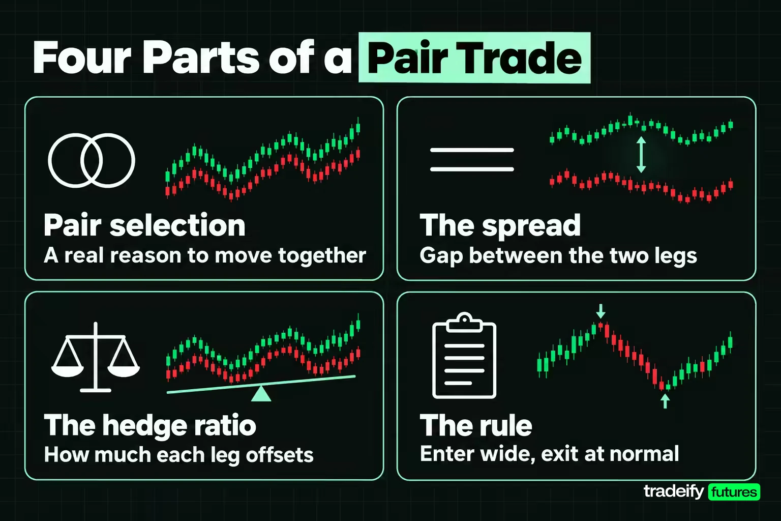
Pairs trading is the two-instrument case of statistical arbitrage and the place the strategy started. You choose two instruments that share a driver, such as two stock index futures, two precious metals or a crude oil contract and a refined product, and you track the gap between them.
A pair trade has four moving parts:
- Pair selection. The two instruments need an economic reason to move together, not just a correlation that happened to show up in one sample.
- The spread. Usually the log price of one leg minus a multiple of the log price of the other, so the spread is close to flat when the relationship is behaving.
- The hedge ratio. That multiple, often called beta, sets how much of the second leg offsets each unit of the first. Get it wrong and the position is a directional bet wearing a spread costume.
- The rule. When the spread is unusually wide, buy the cheap leg and sell the rich one; exit when the spread returns to normal, when a stop is hit, or when time runs out.
The best-known academic test is Gatev, Goetzmann and Rouwenhorst's study of US stocks from 1962 through 1997. They matched stocks into pairs by minimum distance between normalized price paths, traded them over six-month periods, and found average annualized excess returns of up to 12 percent for portfolios of top pairs. That result is the reason pairs trading moved from trading-desk folklore into textbooks.
Statistical arbitrage is what happened when firms widened the idea. Instead of a fixed pair chosen by eye, a model scores many instruments against each other or against common factors, and the portfolio holds many small offsetting positions at once. A two-contract spread with a rolling regression is a scaled-down version of the same machine, with one important difference: it has nowhere to spread the risk when its single relationship breaks.
Mean Reversion and the Z-Score Behind Stat Arb Signals
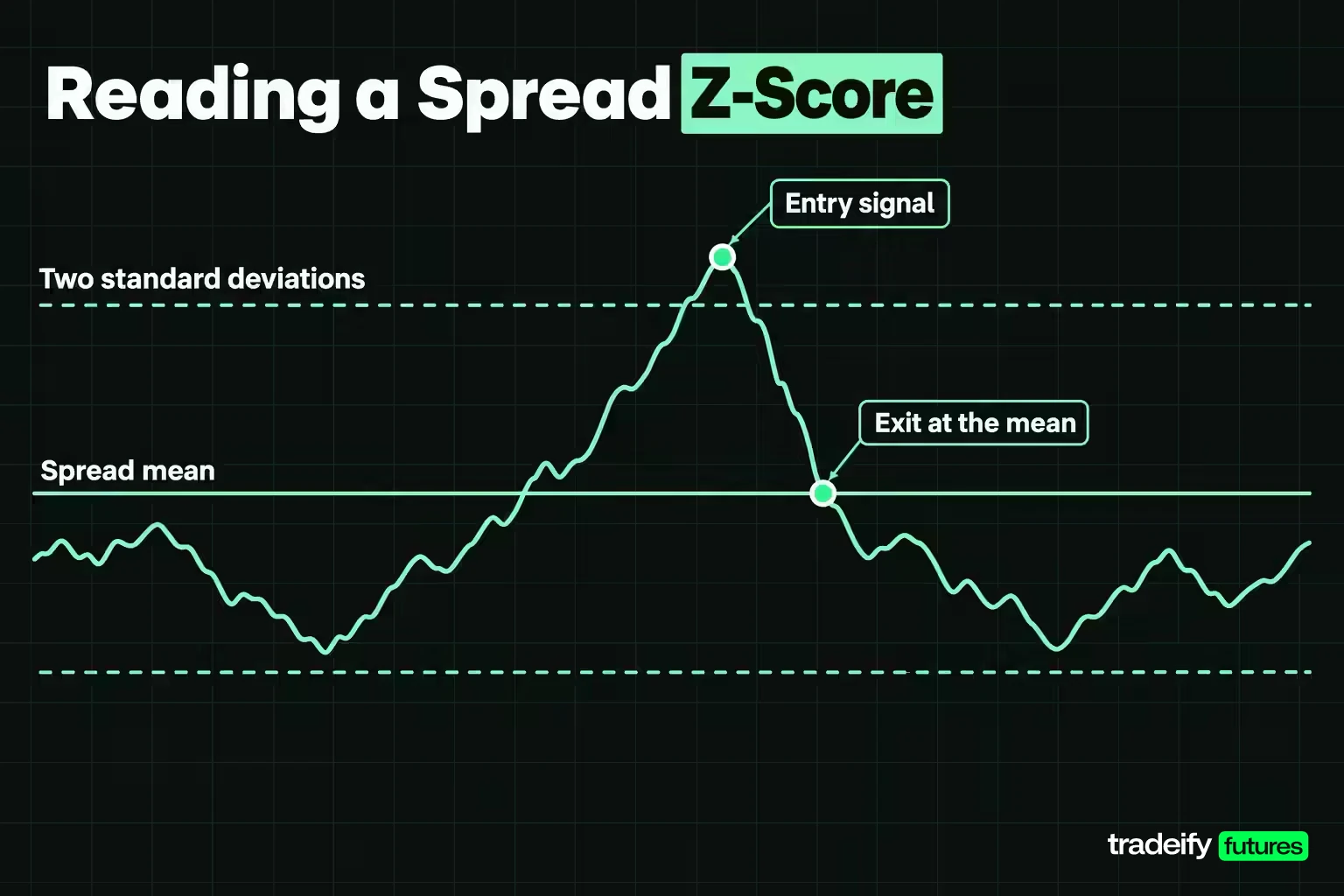
Mean reversion in statistical arbitrage refers to the spread, not to either price. Gold can rally for a year while the spread between gold and silver oscillates around a stable level. The bet is on that oscillation.
To measure how stretched a spread is, most stat arb rules use a z-score. You fit a regression of one leg's log price on the other's over a trailing window, take today's residual (how far today's spread sits from the fitted line), and divide it by the standard deviation of the residuals in that window. A z-score of 2.0 means the spread is two standard deviations from where the relationship says it should be.
Stationarity, cointegration and half-life in a stat arb spread
Three ideas sit underneath the z-score:
- Stationarity. The spread has to keep returning toward a stable mean for the z-score to mean anything. A spread that trends just keeps producing wider readings.
- Cointegration. Two prices can each wander while a combination of them stays stationary. Testing for that, for example with an Engle-Granger two-step test, is a stronger screen than correlation, which only says the daily moves line up.
- Half-life. If you model the spread as reverting at a constant rate, the half-life is the number of sessions it takes to close half of a given gap. A 16-session half-life suits a short hold. A 41-session half-life does not.
Entry thresholds and invalidation for a stat arb z-score
The z-score also tells you what would prove the setup wrong. If the spread keeps widening past the level you would ever expect from the residual history, the more likely explanation is that the relationship changed, not that the opportunity got better. A stat arb rule needs that invalidation level written down before entry, because the temptation once you are in is to read a wider spread as a better price.
How far apart is far enough to enter? There is no universal number. A higher threshold produces fewer, more extreme signals that tend to need a wider stop; a lower one produces more trades with smaller gaps that commissions eat into. Treat the entry threshold and the stop as one decision, because a spread that has already stretched two standard deviations can easily stretch two more before it turns.
Related lesson: Mean reversion trading
Basket Trading and Factor-Neutral Statistical Arbitrage
Basket trading is the step that turns a pair into a portfolio. Instead of comparing one instrument with one other, a basket model compares each instrument with a group, or with the common factors that drive the group, and trades the part of its move the group does not explain.
Two common designs:
- Sector or ETF residuals. Each stock's return is regressed on its sector fund. The leftover return is treated as a mean-reverting signal: buy stocks that lagged their sector, sell those that ran ahead.
- Principal component residuals. A statistical method extracts the few factors that explain most of the co-movement across a universe, then trades each instrument's residual against those factors.
The advantage is diversification of model error. In a basket of a few hundred long and short positions, one broken relationship is a small fraction of the book, and market, sector and factor exposure can be held near zero. That is the form most professional stat arb takes.
The evidence also shows how hard the edge is to keep. Avellaneda and Lee's study of US equities found that, after transaction costs, principal-component strategies produced an average annual Sharpe ratio of 1.44 from 1997 to 2007, but only 0.9 during 2003 to 2007, and the sector-ETF version (1.1 over the full period) degraded in the same way after 2002. When many firms trade the same residuals, the residuals close faster and pay less.
A basket is out of reach for most individual traders because it needs data on many instruments, borrow for the short side, and costs low enough to trade small edges frequently. That is why individual stat arb traders usually end up with the two-leg spread form, and why its single-relationship risk deserves a closer look.
How the Statistical Arbitrage Measurement Was Built
Most explanations of statistical arbitrage stop at the premise that dislocations revert. This measurement checks how often they did, and what happened on the way, on five daily futures spreads. The figures are an illustrative historical study computed for this guide, not a forecast and not a trading system.
Statistical arbitrage study method
- Data. Continuous front-month daily closes from Yahoo Finance for ten CME Group futures, December 31, 2014 to November 4, 2026. Each spread uses the sessions where both legs have a close, about 2,978 per spread, and 2,976 sessions were common to all ten contracts. The series are not back-adjusted, so roll jumps are included as returns, which a trader rolling real contracts would not earn or lose in the same way.
- Spreads. E-mini S&P 500 against E-mini Nasdaq-100, gold against silver, WTI crude oil against RBOB gasoline, 10-Year T-Note against 30-Year T-Bond, and euro FX against British pound futures. Sessions where either close was not positive are excluded, which removes April 20, 2020 from the crude oil spread.
- Spread and z-score. Every session, an ordinary least squares regression of the first leg's log price on the second leg's over the trailing 252 sessions gives the hedge ratio (beta), the intercept and the residual standard deviation. The z-score is the day's residual divided by that standard deviation. The first measured session is December 30, 2015.
- Signal. A signal fires when the absolute z-score reaches 2.0 and no position is open. After an exit, the spread must come back inside 1.0 standard deviation before it can signal again.
- Direction. A positive z-score means the first leg is rich, so the trade sells it and buys the second leg. A negative z-score does the opposite.
- Frozen yardstick. Beta, intercept and standard deviation are frozen at entry, so the whole trade is judged against the relationship that triggered it.
- Exit. The first of three events: the frozen z-score crosses zero (the spread recrosses its mean), the z-score reaches the stop width, or 60 sessions pass.
- Weights and cost. The first leg gets a weight of 1/(1+beta) and the second beta/(1+beta), so results are quoted in basis points of gross exposure. Each trade is charged 6 basis points of gross exposure for the round turn on both legs.
The five futures spreads in the stat arb study
| Spread | Correlation of daily returns | One spread SD (median) | Half-life in sessions | Median beta | Median 60-session beta change |
|---|---|---|---|---|---|
| E-mini S&P 500 vs E-mini Nasdaq-100 | 0.930 | 1.39% | 31.6 | 0.715 | 9.0% |
| Gold vs silver | 0.774 | 3.08% | 41.0 | 0.487 | 21.2% |
| WTI crude oil vs RBOB gasoline | 0.700 | 5.89% | 16.4 | 0.756 | 14.3% |
| 10-Year T-Note vs 30-Year T-Bond | 0.881 | 0.45% | 27.7 | 0.523 | 8.6% |
| Euro FX vs British pound | 0.632 | 1.20% | 30.4 | 0.729 | 24.6% |
The crude oil and gasoline spread is the noisiest, with one standard deviation worth 5.89% of the log spread, and also the fastest, with a 16.4-session half-life. Gold against silver reverts slowest at 41.0 sessions. The euro against the pound has the weakest correlation, 0.632, so a lot of its movement is something the hedge ratio cannot explain.
The beta column is the quiet risk in this statistical arbitrage set. On the currency spread the median hedge ratio moved 24.6% over 60 sessions, and over the whole sample it ranged from -0.093 to 1.512. Gold against silver ran from 0.035 to 1.356. A position sized on one beta and held while beta moves by a fifth is no longer the position you sized.
How Often a Stat Arb Signal Converges
Before adding any stop, the first question for statistical arbitrage is whether a two-sigma dislocation came back at all. This guide's five-spread futures study (Yahoo Finance daily closes, December 31, 2014 to November 4, 2026; the same z-score rule throughout) tracked every signal with no stop for up to 250 sessions and recorded how far the spread moved against the position before it recrossed its mean.
| Spread | Signals | Recrossed within 60 sessions | Recrossed within 250 sessions | Median sessions to recross | Median adverse excursion in SD |
|---|---|---|---|---|---|
| E-mini S&P 500 vs E-mini Nasdaq-100 | 22 | 27.3% | 70.0% | 66.5 | 3.59 |
| Gold vs silver | 18 | 16.7% | 58.8% | 102.5 | 5.39 |
| WTI crude oil vs RBOB gasoline | 29 | 48.3% | 96.4% | 59 | 3.91 |
| 10-Year T-Note vs 30-Year T-Bond | 26 | 38.5% | 52.0% | 34 | 4.91 |
| Euro FX vs British pound | 35 | 37.1% | 66.7% | 40 | 4.22 |
| All five spreads | 130 | 35.4% | 69.9% | 48 | 4.28 |
The 250-session column uses the 123 signals that had a full 250 sessions of data or recrossed sooner. The median sessions column counts only signals that did recross.
What the stat arb convergence rates mean for holding time
In this guide's five-spread study, read the 60-session and 250-session columns together. Within 60 sessions, about three months of trading, 35.4% of statistical arbitrage signals came back to the mean. Allow a full year and 69.9% did, which still leaves almost a third of signals that never resolved inside a year. The premise is true more often than not on a long horizon and false most of the time on the horizon most traders actually hold.
Adverse excursion before a stat arb signal converges
The adverse excursion column is the one that changes position sizing. In the five-spread study, signals entered at 2.0 standard deviations, yet the median signal stretched to 4.28 before recrossing or running out of time, and even the signals that did come back stretched to a median of 3.50 first. 83.8% of signals reached 2.5 standard deviations before they reached the mean. A stop placed just beyond the entry dislocation would have been taken out on most trades that eventually worked.
The excursions are also lopsided. The worst came on the index spread: a signal on January 29, 2020 entered at -2.08 and stretched to 36.61 standard deviations as the Nasdaq-100 pulled away from the S&P 500 through 2020. That is not noise around a mean. It is a relationship changing while the trade was open.
Choosing a Stop Width for Statistical Arbitrage
A stat arb exit can only collect the recross if the position survives long enough to see it. This stop ladder comes from this guide's five-spread futures study (Yahoo Finance daily closes, 2014 to 2026) and runs the full rule (signal at 2.0, exit at the mean recross, a stop at the stated width, or 60 sessions) at six stop widths.
| Stop width in SD | Trades | Stopped | Exited at mean | Exited on time | Winning trades | Average result bp | Median result bp | Worst trade bp | Median hold sessions |
|---|---|---|---|---|---|---|---|---|---|
| 2.5 | 113 | 84.1% | 15.0% | 0.9% | 15.9% | 11.8 | -43.1 | -398.1 | 5 |
| 3.0 | 108 | 64.8% | 22.2% | 13.0% | 28.7% | 21.8 | -51.7 | -930.9 | 14.5 |
| 3.5 | 100 | 50.0% | 26.0% | 24.0% | 36.0% | 14.1 | -50.0 | -930.9 | 25 |
| 4.0 | 99 | 36.4% | 31.3% | 32.3% | 45.5% | 24.8 | -27.1 | -939.9 | 34 |
| 5.0 | 94 | 22.3% | 33.0% | 44.7% | 51.1% | 42.0 | 4.3 | -1,115.4 | 45.5 |
| No stop | 88 | 0.0% | 34.1% | 65.9% | 56.8% | 19.2 | 36.0 | -2,318.6 | 60 |
Tight stops versus wide stops in statistical arbitrage
Two failures show up in the stop ladder. A tight 2.5 stop was hit on 84.1% of trades, so the rule became a stream of small losses with a 15.9% win rate. Wider stops raised the win rate and pulled the median toward zero, but the worst trade grew from -398.1 to -2,318.6 basis points and the median hold stretched from 5 sessions to the full 60.
Trade counts fall as the stop widens because each spread holds one position at a time. A wider stop keeps a losing position open longer, which skips signals that would otherwise have been taken.
In this sample the 5.0 width had the best average and median. Treat that with care. It is one historical path through five spreads, the difference between rows rests on a few large trades, and the widest stops are exactly the ones that let a broken relationship do the most damage. The decision a stop ladder actually supports is narrower: pick the width from your spread's measured adverse excursion and the largest loss you can absorb, then accept the win rate that comes with it.
Related lesson: Backtesting a trading strategy
Why Average Stat Arb Results Hide a Losing Median
In this guide's five-spread futures study, 100 statistical arbitrage trades at the 3.5 standard deviation stop averaged 14.1 basis points. The median trade lost 50.0. The five best trades added 6,590 basis points between them against a net total of 1,406 for the whole set, and removing them turned the average to -54.6.
| Spread at the 3.5 SD stop | Trades | Winning trades | Average result bp | Median result bp |
|---|---|---|---|---|
| E-mini S&P 500 vs E-mini Nasdaq-100 | 18 | 27.8% | -12.3 | -61.1 |
| Gold vs silver | 16 | 37.5% | -54.0 | -93.4 |
| WTI crude oil vs RBOB gasoline | 23 | 39.1% | 115.3 | -208.0 |
| 10-Year T-Note vs 30-Year T-Bond | 18 | 38.9% | -1.9 | -20.5 |
| Euro FX vs British pound | 25 | 36.0% | -5.1 | -59.3 |
Only one of the five spreads had a positive average at that stop, and even there the median trade lost 208.0 basis points. The pooled result is positive because the energy spread produced a few very large winners. A trader running any one of the other four spreads with this rule would have finished behind.
The concentration has a structural reason. A spread that reverts has a bounded gain, because it can only travel from the entry dislocation back to the mean. A spread whose relationship breaks has no equivalent ceiling. The worst trade in the 3.5 set came from crude oil and gasoline: a signal on April 9, 2020 bought crude at $22.76 and sold gasoline at $0.6773 a gallon. By April 14, two sessions later, crude was $20.11 and gasoline $0.7200, the stop was hit, and the trade lost 930.9 basis points, roughly 66 times the average result. Six days later, on April 20, 2020, front-month WTI crude oil futures traded below zero for the first time.
That is what sizing has to be built around. A position sized for a 14.1 basis point edge will not survive a 930.9 basis point loss unless it was small to begin with, and a backtest that happened to skip that one month would never show you the risk.
Related lesson: Risk of ruin
Does a Statistical Arbitrage Signal Beat a Random Entry
A fair challenge to any convergence rule is that spreads wander, so a bet on convergence might earn something whether or not the signal means anything. This test, from this guide's five-spread futures study (Yahoo Finance daily closes, 2014 to 2026), compares two-sigma signal sessions with all other sessions on the same spreads, in the same convergence direction, over the same 60-session hold with no stop, sampled every five sessions.
| Spread | Signal samples | Signal average bp | Signal median bp | Other sessions average bp | Other sessions median bp |
|---|---|---|---|---|---|
| E-mini S&P 500 vs E-mini Nasdaq-100 | 66 | 45.6 | 96.0 | 23.8 | 26.4 |
| Gold vs silver | 75 | 197.7 | 197.0 | -88.7 | -59.4 |
| WTI crude oil vs RBOB gasoline | 45 | 649.2 | 228.4 | 146.8 | 100.4 |
| 10-Year T-Note vs 30-Year T-Bond | 84 | -15.2 | -22.9 | -9.1 | -5.5 |
| Euro FX vs British pound | 79 | 33.8 | 20.7 | 3.3 | -13.6 |
| All five spreads | 349 | 138.8 | 20.7 | 17.1 | 1.9 |
Pooled across 349 signal samples and 2,321 other samples, signal sessions averaged 138.8 basis points against 17.1, and the median was 20.7 against 1.9. 53.6% of signal samples finished positive against 50.8% of the others. The naive t-statistic on the difference in averages is 3.14, but adjacent 60-session windows sampled five sessions apart share 55 sessions, so that figure overstates the confidence. Treat it as directional evidence, not proof.
The per-spread rows matter more than the pooled line. Four spreads did better after a signal than at an arbitrary session. The Treasury spread did worse after a signal, and the pooled average leans heavily on the energy spread. So the threshold carried some information in this sample, but a pooled test tells you a method can work on a data set. It does not tell you which spread you are about to trade.
A Statistical Arbitrage Trade Worked Through in Dollars
Numbers are easier to trust when you can follow one statistical arbitrage trade. This is the first E-mini S&P 500 against E-mini Nasdaq-100 trade that exited at the mean in this guide's five-spread study (2.0 entry, 3.5 standard deviation stop, 60-session cap, Yahoo Finance daily closes), chosen by its position in the trade log rather than its outcome.
On June 16, 2022 the spread reached a z-score of -2.30, meaning the S&P 500 contract looked cheap relative to the Nasdaq-100 contract. The frozen beta was 0.540, so the rule bought the S&P leg with 64.9% of gross exposure and sold the Nasdaq leg with 35.1%. The spread stretched to -2.39 at worst, never threatened the 3.5 stop, and recrossed its mean on July 29, 2022, 29 sessions later.
| Leg on $10,000 gross | Entry close June 16, 2022 | Exit close July 29, 2022 | Price change | Position | Result |
|---|---|---|---|---|---|
| E-mini S&P 500 | 3,668.25 | 4,133.50 | +12.68% | Long $6,492 | +$823 |
| E-mini Nasdaq-100 | 11,124.75 | 12,971.50 | +16.60% | Short $3,508 | -$582 |
Why the hedge ratio decided this stat arb trade
In the June 2022 index spread trade, the two legs net to about +$241, and the 6 basis point cost on $10,000 takes $6, leaving $235. Both legs rose, and the Nasdaq leg rose further. The trade still made money because the hedge ratio said the Nasdaq leg only needed to be about half the size of the S&P leg. An equal-dollar version of the same idea, $5,000 on each side, would have lost about $196 before costs. In statistical arbitrage the hedge ratio is not a detail. It decides whether the trade is a spread or a bet on which index goes up more.
In spread terms, one standard deviation was worth about 1.01% of gross exposure on the June 2022 trade. The move from entry back to the mean was worth about 2.31%, and the 3.5 stop sat about 1.21% away. That is roughly $231 of target against $121 of stop on $10,000 gross. This one went the trader's way after stretching only 0.09 standard deviations past its entry, which is the exception: the median signal in the five-spread study stretched more than two full standard deviations past its entry first.
Contract size and the stat arb hedge ratio
Contract size limits how precisely a trader can express a statistical arbitrage hedge ratio. At the June 16, 2022 entry prices of 3,668.25 and 11,124.75, one E-mini S&P 500 contract ($50 per point) carried $183,412.50 of notional and one E-mini Nasdaq-100 contract ($20 per point) carried $222,495, so the closest full-size ratio was far from 0.540. With micros it gets closer: 9 Micro E-mini S&P 500 contracts ($5 per point) came to $165,071.25 and 4 Micro E-mini Nasdaq-100 contracts ($2 per point) to $88,998, a ratio of 0.539. Real positions carry real notional, and a futures spread of this size can lose far more than the basis points on a $10,000 illustration suggest.
Related lesson: Position sizing futures contracts
Statistical Arbitrage Risks and Challenges
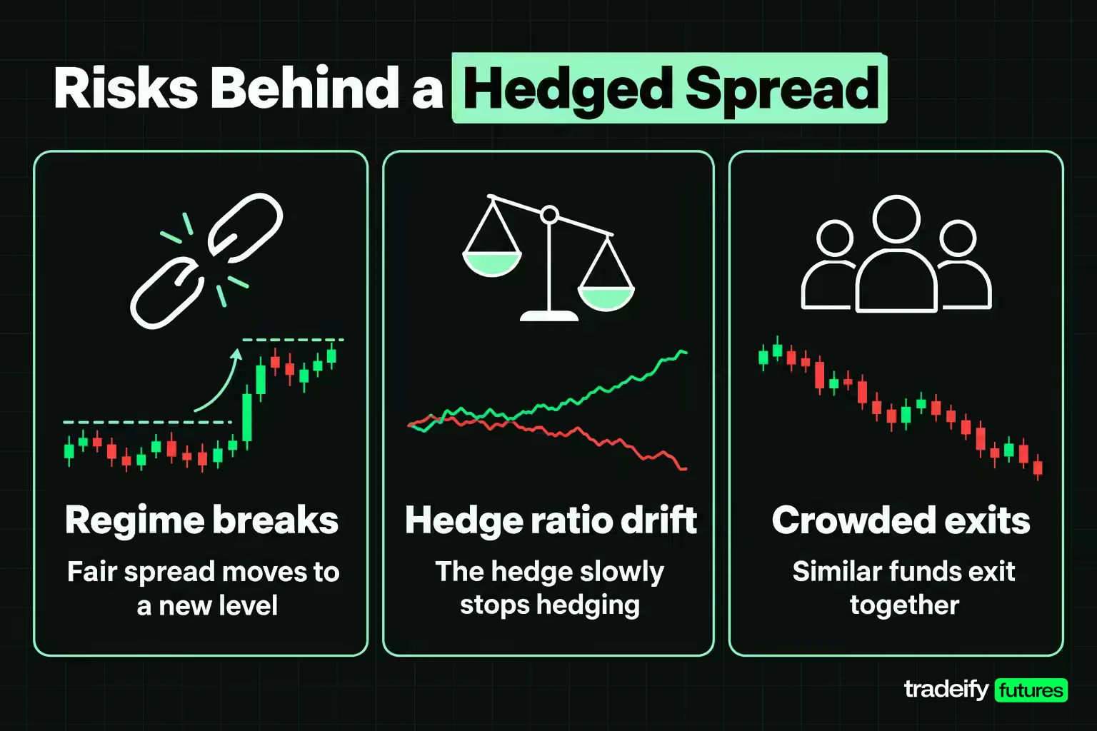
Statistical arbitrage is often described as low risk because it is hedged. The hedge removes market direction from the trade, and in exchange you take on risks that a one-legged trader never has to think about.
Model risk and regime breaks in stat arb
Every stat arb signal assumes the relationship in the lookback window still holds. Regime breaks (a change in monetary policy, a supply shock, a sector rotation) can move the fair spread to a new level. When that happens, the trade is not early. It is wrong, and the z-score keeps widening because it is measured against the old relationship. In this guide's five-spread study, an S&P 500 against Nasdaq-100 signal from January 29, 2020 stretched to 36.61 standard deviations: that failure in numbers.
Hedge ratio drift in a stat arb spread
The hedge ratio in a stat arb spread is an estimate, and it moves. In this guide's five-spread futures study (Yahoo Finance daily closes, 2014 to 2026), the median 60-session change in beta ran from 8.6% on the 10-Year against 30-Year Treasury spread to 24.6% on the euro against pound spread. Refit the beta and the position changes size and exposure; freeze it and the hedge slowly stops hedging. Neither choice removes the risk. You have to decide which one your rule accepts.
Crowding and correlated stat arb exits
Khandani and Lo studied the week of August 6, 2007, when a number of quantitative long and short equity hedge funds lost heavily at the same time. Their analysis points to a fast unwind of one large portfolio hitting other funds that held similar positions, and earlier simulations by the same authors showed returns to simple stat arb strategies falling from 1998 to 2007 as more capital chased them. When a spread is popular, its exit is shared.
Funding, margin and stat arb holding time
A correct convergence call can still lose if the position cannot be held until it converges. Long-Term Capital Management's failure in 1998 is the textbook case of a fund unable to post collateral against adverse moves. On a smaller scale, the same mechanism applies to any statistical arbitrage trader whose margin, drawdown limit or patience runs out before the spread turns. In this guide's five-spread futures study, the median two-sigma signal took 48 sessions to recross when it recrossed at all.
Costs, slippage and the short leg in stat arb
A stat arb edge is small per trade, so costs eat a large share of it. Two legs mean two sets of commissions, two bid-ask spreads and twice the chance of a bad fill when one leg gaps. Shorting stocks adds borrow fees and recall risk. A backtest that charges a fixed cost, such as the 6 basis points per round turn used in this guide's five-spread study, understates real costs, which widen exactly when spreads are stretched and markets are fast.
Related lesson: Correlation risk
Technology, Speed and Machine Learning in Stat Arb
A working statistical arbitrage process needs three layers of infrastructure. Each one is a place where a backtest and live trading can disagree.
- Data. Clean, aligned price history for every instrument, with roll handling for futures, corporate actions for stocks, and enough history to estimate the relationship and test it on data the model never saw.
- Research. A backtesting engine that refits parameters using only data available at each point in time, charges realistic costs, and reports the distribution of results, not only the average. Walk-forward or out-of-sample testing guards against fitting the noise of one sample.
- Execution. Order routing that can fill both legs close together, position and risk monitoring, and a kill switch. For manual traders, a platform that can place both legs and track the spread's z-score in real time.
High-frequency and cross-exchange statistical arbitrage
High-frequency statistical arbitrage runs the same logic on seconds or milliseconds rather than days: tiny dislocations between related instruments, closed quickly, many thousands of times. Its edge depends on speed, colocated servers and very low costs, which puts it out of reach for individual traders. Cross-exchange arbitrage, common in crypto, trades the same asset quoted at different prices on two venues: buy where it is cheaper, sell where it is dearer, and capture the gap. That is closer to true arbitrage than stat arb, because the two prices refer to the same asset. Where it fails is in the plumbing. Moving coins or cash between venues takes time while the gap can close, withdrawal limits and fees eat the margin, and holding balances on several exchanges adds counterparty risk if a venue halts withdrawals. Traders who pre-fund both venues avoid the transfer delay but tie up capital on each one. Derivatives arbitrage trades the relationship between a derivative and its underlying, such as a futures contract against its cash index; it relies on fixed pricing relationships rather than statistical ones, and those gaps are usually closed by large firms within moments.
Machine learning in statistical arbitrage
Machine learning has become a common way to score stat arb candidates. Krauss, Do and Huck trained deep neural networks, gradient-boosted trees and random forests on lagged returns of S&P 500 stocks from 1992 to 2015 and bought the top 10 and sold the bottom 10 each day. An equal-weighted ensemble of the three models averaged 0.45 percent per day before transaction costs and 0.25 percent per day after, with profits declining in later years. The lesson cuts both ways: models can find structure, and daily turnover makes costs decisive.
Is Statistical Arbitrage Legal
Yes. Statistical arbitrage is a recognized strategy used by hedge funds, banks and proprietary trading firms, and trading a spread on your own account is ordinary trading.
What is illegal is manipulation. In US futures markets, the Commodity Exchange Act prohibits disruptive practices including "spoofing", defined as bidding or offering with the intent to cancel the bid or offer before execution. A stat arb strategy that places orders it intends to fill is not spoofing; an automated strategy that layers orders to move a price and then cancels them can be.
Regulation changes when you trade other people's money. In the US, managing or advising on futures accounts for others can require registration, for example as a commodity trading advisor. Separately, brokers and trading programs can set their own rules on hedging, correlated positions and automation that are stricter than the law, so check the rules of the account you trade before assuming a spread is allowed there.
Statistical Arbitrage in Funded Futures Accounts
Funded and evaluation futures accounts are a poor fit for the two-leg form of statistical arbitrage studied in this guide. Many prop firms restrict holding opposing positions in correlated products because a long and short pair can be used to game drawdown rules, and many require positions to be closed before the end of each session. A spread that needs weeks to converge cannot be held under an intraday rule, and a long and short pair in two closely related contracts can fall under a hedging rule even when the trader intends it as a genuine spread.
On our accounts, these spreads are not available. Our hedging rule prohibits opposing positions on the same instrument or on two products from the same Product Group, in one account or across accounts, and our Help Center gives long ES with short NQ as an example of a violation; gold and silver both sit in our Metals group, and the euro and pound in Currencies. 10-Year and 30-Year Treasury futures and RBOB gasoline are not on our supported product list, and every position must be closed by 4:45 PM ET, so a multi-week spread cannot be carried. Our funded accounts are simulated.
What carries over to directional intraday trading is the measurement habit. Logging the adverse excursion on every trade, comparing the average with the median, and checking how much of a result rests on a few trades are useful on any strategy.
A Statistical Arbitrage Checklist Before You Trade a Spread
Use this checklist before putting money behind any statistical arbitrage spread, whatever account it runs in.
- Measure the recross rate on your own spread and holding period. In this guide's five-spread futures study the 60-session rate ran from 16.7% to 48.3%. A pooled rate from someone else's data is not your number.
- Size the stop from the adverse excursion, not the entry threshold. In the same study, the median signal stretched to 4.28 standard deviations. A stop just beyond 2.0 will be hit on most trades.
- Watch beta while you hold. If the hedge ratio has moved by a fifth, re-check what the position is now exposed to.
- Report the average with and without the five best and five worst trades. If the result depends on five trades, size for the tail you have not seen yet.
- Price your real costs. Two legs, two spreads, two commissions. Re-run the test with costs doubled and see what is left.
- Decide the time cap before entry. In this guide's five-spread study with no stop, 65.9% of trades ended on the 60-session cap rather than at the mean.
- Check the account rules. Hedging, correlated-product and overnight rules can make a spread unavailable before the market gets a vote.
Statistical Arbitrage FAQ
What is statistical arbitrage in simple terms?
It is trading the gap between related instruments and betting that the gap returns to normal. You buy the one that looks cheap relative to the relationship and sell the one that looks rich. The expected profit is statistical, not locked in, and the gap can widen or never close.
Is statistical arbitrage the same as pairs trading?
Not exactly. Pairs trading is the two-instrument case, usually with a chosen pair. Statistical arbitrage is the wider family and usually uses a model across many instruments or factors, with a risk model to strip out common exposure.
Is arbitrage trading illegal?
No. Statistical arbitrage on your own account is legal. Manipulation such as spoofing is illegal, and individual brokers or trading programs may ban specific hedged or correlated positions under their own rules.
Can you really make money with statistical arbitrage?
Some firms have, and published studies show the edge shrinking as more capital chased it. In this guide's five-spread futures study (Yahoo Finance daily data, 2014 to 2026), the pooled average statistical arbitrage trade was positive at every stop width tested. But the median trade lost at four of the six widths, and the average at the 3.5 width rested on five trades.
How risky is statistical arbitrage?
Statistical arbitrage is riskier than the hedge suggests. In this guide's five-spread futures study, signals stretched to a median of 4.28 standard deviations against a 2.0 entry, and the worst trade at the 3.5 stop lost 930.9 basis points when a relationship broke. Crowding, margin calls and two-leg execution add to that.
What are the three types of arbitrage?
A common breakdown is pure arbitrage (the same asset at two prices at once), risk or merger arbitrage (a bet on a deal closing), and statistical arbitrage (a bet on a historical relationship). Only the first comes close to locking in a profit, and even it carries execution risk.
How long does a statistical arbitrage trade take to work?
Usually longer than traders expect. In this guide's five-spread futures study, signals that recrossed their mean took a median of 48 sessions, and only 35.4% did so within 60 sessions. Stopped trades at the 3.5 width were out in a median of 11 sessions, so losses arrived faster than wins.
This guide is educational and is not investment, legal or tax advice, or a recommendation to trade any instrument. Futures and leveraged spread positions can lose on both legs at once and can lose more than expected, and hedge ratios, volatility and correlations change over time. The study describes one historical sample of five futures spreads, uses non-back-adjusted continuous data and a fixed cost assumption, and is not a forecast. Funded and evaluation accounts are simulated, and trading program rules differ and can change. Trade only with money you can afford to lose.


