




TL;DR: Correlation risk is the chance that positions you sized as separate bets lose together, so total risk exceeds what the count implies. On 20 years of ES, NQ, gold, silver and copper futures, ES and NQ ran at 0.92 and the ten pairs averaged 0.34. At that average, five positions carried 54% more combined risk than the independence shortcut assumes. Correlation also moved a lot, so measure it on rolling windows and size the whole book, not each trade.
Correlation risk shows up the day three "different" trades all hit their stops before lunch. Each position was sized correctly on its own. The problem was that they were never really three positions.
It usually starts with a reasonable thought. You like the long ES setup, NQ looks just as good, and taking both feels like spreading the bet. On the chart they are two trades. In your account, on most days, they are one.
This guide explains what correlation measures, how it differs from covariance, and how it changes the risk of a book of futures positions. Every claim about how markets behave is tested on a 20-year measurement of five futures markets, so you can see the numbers rather than take the usual warnings on faith.
What Correlation Risk Means
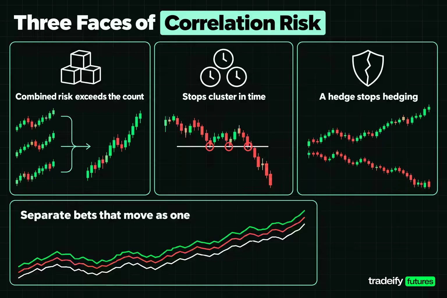
Correlation risk is the risk that positions you treat as separate move as one. It is not a statement about direction or volatility. Two quiet markets can travel together, and two wild markets can cancel each other out.
NYU Stern's V-Lab correlation documentation puts the stakes plainly: correlations decide how much diversification benefit a portfolio gets, how well a hedge works, and how much risk you are actually taking when you think it is spread out.
For a trader holding more than one position, correlation risk shows up in three ways, and each has a different fix.
- Combined risk is larger than the position count implies. Five positions at 1% each do not carry the 2.24% of combined risk the independence math gives you when the markets move together.
- Stops cluster in time. If the positions are correlated, the losses arrive on the same session instead of spreading across the month, so the drawdown is faster and deeper.
- A hedge stops hedging. A pair that offset each other for a year can move together the next, and the position meant to reduce risk adds to it.
The rest of this guide puts a number on each one.
Related lesson: Risk management for traders
How the Correlation Coefficient Works
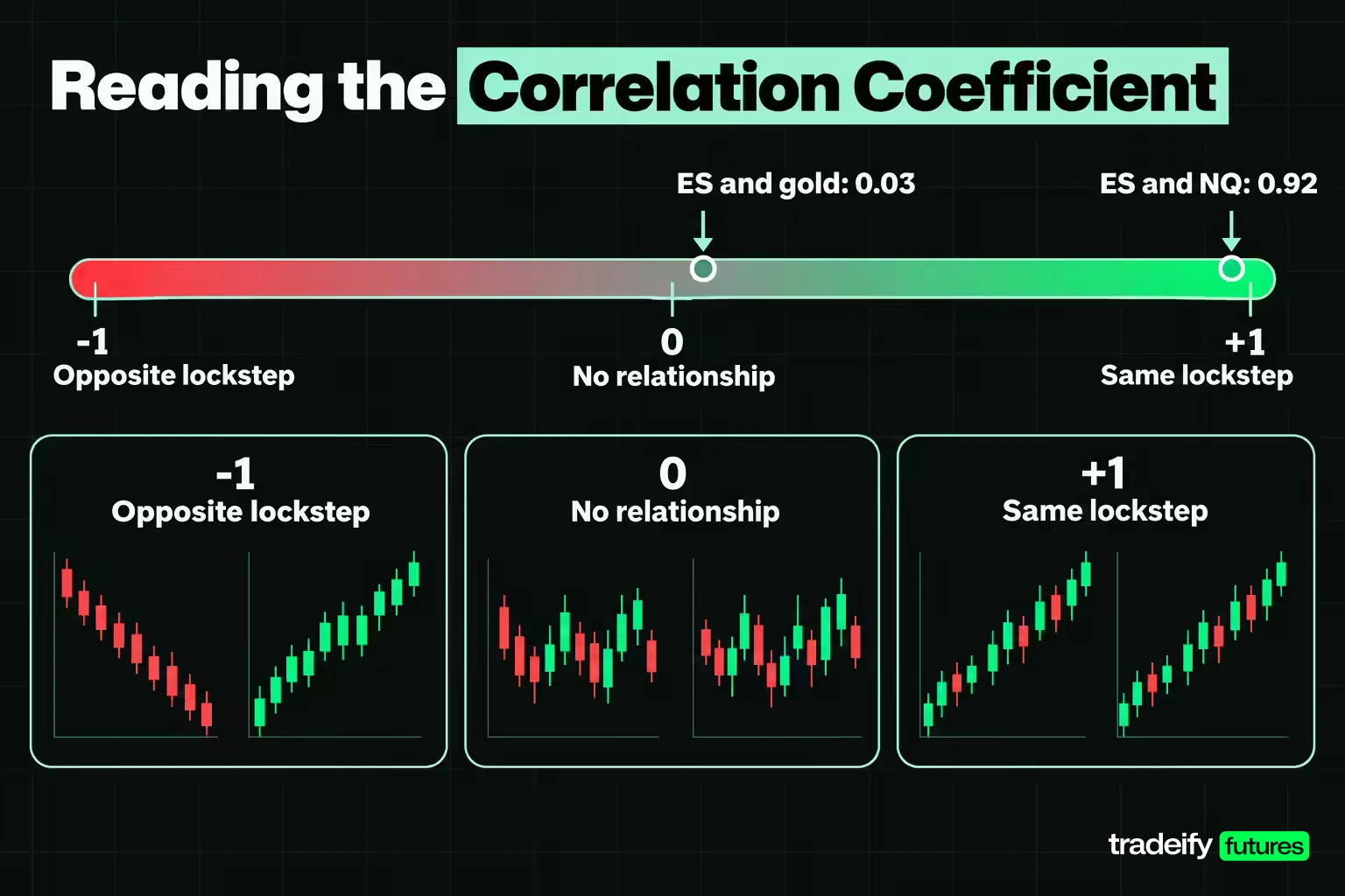
The correlation coefficient, usually Pearson's r, measures how consistently two series move together in a straight-line relationship. It runs from -1 to +1.
- +1 means the two move in perfect lockstep in the same direction.
- 0 means no linear relationship. Knowing one tells you nothing about the other's direction.
- -1 means perfect lockstep in opposite directions.
In practice you rarely see the extremes. On the five futures markets measured below, the E-mini S&P 500 (ES) and E-mini Nasdaq 100 (NQ) ran at 0.92 over 20 years of daily returns, which is about as close to lockstep as two separate contracts get. ES and gold ran at 0.03, which is close to no relationship at all.
Reading correlation values for trading
Rules of thumb that call 0.3 "weak" and 0.7 "strong" come from describing data, not from sizing positions. For risk, a better read is the shared variance, which is the correlation squared (often written R-squared).
At 0.92, about 85.4% of the day-to-day variation in ES returns is shared with NQ. At 0.5, a figure many people call "moderate", 25% is shared, and that is still enough to lift combined risk sharply once you hold several positions. Five positions at a 0.5 average correlation, each risking 1%, carry 3.87% of combined risk instead of 2.24%.
Why correlation uses returns, not prices
Correlation must be computed on returns (the percentage or log change from one close to the next), not on price levels. Prices trend, and any two series that both rose over a decade look related on a price chart even if their daily moves have nothing in common.
A rank-based version, Spearman's correlation, is a useful cross-check. It correlates the order of the returns instead of their size, so a few extreme days carry less weight. On the same data, Spearman's correlation for ES and NQ came out at 0.89 against Pearson's 0.92, and for ES and gold at 0.05 against 0.03. When the two measures agree like this, the relationship is not being driven by a handful of outliers.
Correlation vs Covariance
Covariance and correlation measure the same co-movement in different units. Covariance is the average product of the two series' deviations from their means. The NIST/SEMATECH e-Handbook of Statistical Methods gives the sample formula: the sum of (X minus its mean) times (Y minus its mean), divided by n minus 1.
Correlation is covariance rescaled to a fixed range:
- Correlation = covariance ÷ (standard deviation of X × standard deviation of Y)
- Covariance = correlation × standard deviation of X × standard deviation of Y
That rescaling is the whole difference, and it matters more than it looks.
Why covariance depends on volatility
Covariance carries the units and the volatility of both series. Measured on daily returns in percent, the covariance of ES and NQ is 1.62. The covariance of gold and silver is 2.03, higher than ES and NQ even though the gold and silver correlation is lower, at 0.79.
The reason is silver's volatility. Its daily standard deviation in this sample was 2.22%, against 1.24% for ES, 1.41% for NQ, 1.16% for gold and 1.73% for copper. Covariance rolls that volatility into the number, so you cannot compare covariances across pairs and conclude which pair is more tightly linked.
When to use correlation and when to use covariance
- Use correlation to compare relationships. It answers "which of my positions behave like the same trade?" on one scale for every pair.
- Use covariance, or correlation combined with each position's dollar risk, to compute portfolio risk. The variance of a book is built from covariances, which is why the sizing math later in this guide multiplies each correlation by the two positions' risk.
- Report correlation to people, compute with covariance. A covariance number on its own is hard to interpret. A correlation of 0.92 is not.
Correlation Risk Measured on Five Futures Markets
To put numbers on correlation risk, this guide uses one illustrative study. The data are Yahoo Finance continuous front-month daily bars for five CME Group futures: the E-mini S&P 500 (ES), the E-mini Nasdaq 100 (NQ), gold (GC), silver (SI) and copper (HG). Only sessions with a complete bar in all five markets count, which leaves 5,027 daily log returns from November 6, 2006 to November 4, 2026.
Five markets produce ten pairs, since each pair is counted once, and each pair is a separate source of correlation risk. The full set sits in a correlation matrix: a grid with every market on both axes, 1.00 on the diagonal (each market against itself), and the same value mirrored above and below it.
| Market | ES | NQ | Gold | Silver | Copper |
|---|---|---|---|---|---|
| ES | 1.00 | 0.92 | 0.03 | 0.16 | 0.30 |
| NQ | 0.92 | 1.00 | 0.03 | 0.15 | 0.26 |
| Gold | 0.03 | 0.03 | 1.00 | 0.79 | 0.33 |
| Silver | 0.16 | 0.15 | 0.79 | 1.00 | 0.44 |
| Copper | 0.30 | 0.26 | 0.33 | 0.44 | 1.00 |
Two pairs dominate. ES and NQ at 0.92 are effectively one large equity-index position plus a small relative bet between the two indexes. This is where traders usually get caught: the setups look independent, so the risk feels independent, and the correlation risk only becomes visible on the session both stop out. Gold and silver at 0.79 are the second tight pair. At the other end, both stock indexes against gold sit at 0.03, which is close to no linear relationship over 20 years.
The average of the ten pairs is 0.34. That is the number that matters for a book holding all five, because no single pair describes it.
How to specify a correlation matrix as a risk input
A correlation matrix is only as useful as the choices behind it. Before using one for sizing, pin down:
- The return type. Daily log returns here. Weekly or monthly returns give different numbers, so never mix frequencies inside one matrix.
- The window. A full 20-year sample gives a stable average but hides how much the number moved, which the rolling-window section below measures.
- The alignment. Every market must use the same sessions. Holidays that close one exchange but not another create false zero-return days.
- The sign convention for short positions. A short position flips the sign of its correlation with everything else.
Related lesson: Diversification
How Correlation Changes Portfolio Risk
Correlation enters your risk math in exactly one place: the combined risk of the book. That is why it is easy to miss. Position sizing happens one trade at a time, so each trade looks fine. The error only appears in the total.
The variance-correlation decomposition
For positions with equal risk, where "risk" means each position's typical one-session swing (one standard deviation), combined risk is:
- Combined risk = per-position risk × the square root of (N + N × (N - 1) × average correlation)
N is the number of positions. With zero correlation the formula collapses to the square root of N, which is the shortcut most traders carry in their heads. With a correlation of 1, it becomes N, meaning the positions add up as if they were one.
At the measured average of 0.3426 (0.34 to two decimals), here is what that does to a book where every position risks 1% of the account per session.
| Positions | Combined risk at 0.3426 | Independence shortcut | Gap | Effective independent bets | Per-position risk for 1% total |
|---|---|---|---|---|---|
| 1 | 1.00% | 1.00% | 0% | 1.00 | 1.00% |
| 2 | 1.64% | 1.41% | 15.9% | 1.49 | 0.61% |
| 3 | 2.25% | 1.73% | 29.8% | 1.78 | 0.44% |
| 5 | 3.44% | 2.24% | 54.0% | 2.11 | 0.29% |
| 10 | 6.39% | 3.16% | 102.1% | 2.45 | 0.16% |
Read the last column as the practical answer. To hold a five-position book's combined risk at 1%, each position is sized at 0.29% of the account, not the 0.45% the shortcut allows. That gap is the cost of correlation risk, paid up front in smaller size instead of later in a deeper drawdown.
What would change the answer is the average correlation of the positions you actually hold. Swap NQ for a market with a near-zero correlation to the rest of the book and the same five slots carry noticeably less combined risk. Add a second equity index and it goes the other way.
The diversification ceiling
Effective independent bets equal N ÷ (1 + (N - 1) × average correlation). As N grows, that number approaches 1 ÷ the average correlation and never passes it. At 0.3426, the ceiling is 2.92 independent bets.
That is the uncomfortable part of portfolio diversification. Five positions behave like 2.11 independent bets. Ten behave like 2.45. Adding markets past a handful mostly adds commissions and screen time, unless the new market genuinely has a low correlation with what you already hold.
Lower vs higher correlation in a portfolio
For positions in the same direction, lower is better, because it cuts combined risk and spreads the losses out. Holding the same 1% per position across five markets, combined risk is 2.24% at a correlation of 0, 3.00% at 0.2, 3.87% at 0.5 and 4.36% at 0.7.
For a deliberate long-short spread, the reverse holds. High positive correlation is what makes the spread behave like a bet on the gap between two markets instead of a bet on direction.
Related lesson: Portfolio heat and total exposure
A Worked Correlation Risk Example
Imagine an illustrative $50,000 account holding three long positions: ES, NQ and gold. Each is sized so its typical one-session swing is $500, which is 1% of the account.
Correlation risk on three positions, checked by hand
The three pairwise correlations from this guide's 20-year study of Yahoo Finance futures data are 0.924 (ES and NQ), 0.033 (ES and gold) and 0.035 (NQ and gold). Their sum is 0.992.
- Inside the square root: 3 + 2 × 0.992 = 4.984.
- The square root of 4.984 is about 2.2325.
- Combined risk: $500 × 2.2325 = $1,116, or 2.23% of the account.
The independence shortcut gives $500 × the square root of 3, which is $866, or 1.73%. The measured figure is 28.9% higher.
To hold combined risk at $500, each position would be sized at $224 of typical swing, not the $289 the shortcut allows. The three positions behave like 1.81 independent bets, which matches what the matrix already said: ES and NQ are close to one trade, and gold is the only real second one.
Turning correlation into micro futures contracts
The same math works in contracts. Take one micro of each, at round illustrative prices, and the daily standard deviations measured in the study:
- One MES (Micro E-mini S&P 500, $5 per index point) at an illustrative 7,000 is $35,000 of notional. At a 1.24% daily standard deviation, its typical one-session swing is about $435.
- One MNQ (Micro E-mini Nasdaq-100, $2 per index point) at an illustrative 28,000 is $56,000 of notional, with a typical swing of about $790 at 1.41%.
- One MGC (Micro Gold, 10 troy ounces) at an illustrative $4,000 per ounce is $40,000 of notional, with a typical swing of about $464 at 1.16%.
One MES and one MNQ together swing about $1,203 on a typical session. That is close to the $1,225 you would get by simply adding the two, because at 0.92 they barely offset each other. Adding the MGC lifts the total to about $1,305, only $101 more, despite adding a $464 position. That gap between the two additions is what low correlation buys you.
Related lesson: Position sizing
Correlation in Risk Management and VaR
Correlation is built into the standard risk numbers, starting with value at risk (VaR), so correlation risk sits inside every VaR figure whether or not anyone names it. VaR estimates the loss a position or book should exceed only rarely, for example on 5% of sessions. V-Lab's documentation notes that a bank's VaR depends on assumed correlations between asset classes, and that losses can be much larger than expected if those correlations shift.
Historical VaR with and without correlation
This guide's 20-year study gives historical one-day 95% VaR figures (the loss exceeded on the worst 5% of sessions) that show the effect directly. Each figure is a percentage of one leg's notional, so a pair of equal legs is compared with the two single-leg figures added together.
| Position | One-day 95% historical VaR | Sum of the single legs |
|---|---|---|
| ES alone | 1.82% | Not applicable |
| NQ alone | 2.24% | Not applicable |
| Gold alone | 1.83% | Not applicable |
| ES plus NQ, equal notional | 3.96% | 4.06% |
| ES plus gold, equal notional | 2.65% | 3.65% |
ES plus NQ gets almost no benefit from being two positions. Its VaR is 3.96%, nearly the 4.06% you would get by adding the two legs. ES plus gold, with near-zero correlation, comes in a full point lower than the sum of its legs.
How often everything loses on the same session
VaR describes one bad day. Correlation risk also shows up in how often every position loses together.
In this guide's 20-year study of Yahoo Finance daily futures data for ES, NQ, gold, silver and copper, all five markets closed lower on the same session 603 times, or 12.0% of sessions. Each market fell on roughly 44% to 49% of sessions, so if they were independent, all five would fall together on about 2.2% of sessions. The observed rate is 5.5 times that.
In the same study, on the worst 5% of sessions for an equal-weight basket of all five, every market fell together 71.7% of the time. That is the session that turns five separate stop losses into one large one, and it is correlation risk at its most expensive.
Why this matters for a daily loss limit
Many traders work under a daily loss limit, either their own or one set by a firm. Correlation decides whether that limit holds. Five positions with stops at 1% each can lose 5% on one session if all five stop out, and in this guide's 20-year study of ES, NQ, gold, silver and copper, all five fell together on 12.0% of sessions, far more often than the 2.2% independence suggests. The working rule is to size so that the simultaneous stop-out of every correlated position still lands inside the daily limit.
Related lesson: Tail risk and black swan events
Why Correlation Is Not a Constant
Every correlation quoted so far is an average over 20 years, and no trader trades an average. Correlation risk lives in the current window, not the long-run figure. To see the range, the study recomputed the matrix on 4,968 overlapping windows of 60 sessions each, about three months of trading.
In this guide's study of Yahoo Finance daily data, the average of the ten pairs ran from -0.01 in the window ending November 27, 2019, to 0.73 in the window ending January 23, 2012, with a median of 0.34. It sat above 0.60 in 5.1% of windows and below 0.20 in 17.4% of them.
The pair detail is where the decisions sit:
| Pair | 5th percentile | Median | 95th percentile | Windows below zero |
|---|---|---|---|---|
| ES and NQ | 0.81 | 0.93 | 0.97 | 0.0% |
| Gold and silver | 0.67 | 0.82 | 0.90 | 0.0% |
| Silver and copper | 0.08 | 0.48 | 0.71 | 2.9% |
| ES and copper | -0.01 | 0.30 | 0.61 | 5.4% |
| ES and gold | -0.39 | 0.03 | 0.48 | 46.2% |
In the same 20-year study, ES and NQ never went negative in 60-session windows, and their 5th percentile was still 0.81. That pair is one position all the time. ES and gold went negative in 46.2% of windows, so a book that counted on gold to offset stocks was relying on a coin toss.
Does the window length change the answer
Shorter windows swing more, longer windows less, but the conclusions of this guide's 20-year study held. For ES and gold, the share of negative windows was 46.2% at 20 sessions, 45.2% at 120 sessions and 44.2% at 250 sessions. For ES and NQ, the 5th percentile was 0.76 at 20 sessions and 0.85 at 250 sessions. No window length turns ES and NQ into two positions, and none makes gold a reliable stock hedge.
Five-market correlation as of November 4, 2026
As of November 4, 2026, this guide's study put the 60-session average across the five markets at 0.56, higher than 91.9% of all windows since 2006. In that same window ES and gold measured 0.49, near the top of that pair's range. This is a dated snapshot and will move, but it shows why a correlation looked up once is not the correlation running today.
Related lesson: Hedging risk
Does Correlation Rise in a Crisis
The common claim is that "correlations go to one" when markets fall. This sample supports a narrower version of it, and the difference changes what you should prepare for.
Correlation by volatility regime
Sorting the 4,968 windows by ES's trailing 20-session realized volatility and splitting them into five equal groups gives:
| ES volatility group | Annualized volatility range | Average correlation of the ten pairs |
|---|---|---|
| Calmest fifth | 3.0% to 8.9% | 0.28 |
| Second fifth | 8.9% to 11.9% | 0.35 |
| Middle fifth | 11.9% to 15.5% | 0.37 |
| Fourth fifth | 15.5% to 20.9% | 0.38 |
| Most volatile fifth | 20.9% to 95.4% | 0.33 |
In this guide's study, correlation does rise from calm markets to busy ones. It does not keep rising into the most volatile stretch, and it never got anywhere near 1.
Direction agreement on the worst sessions
What does jump is agreement on direction. In this guide's study of the five futures markets, 62.7% of the ten pairs closed in the same direction on an average session. On the worst 5% of basket sessions, 87.3% did. ES and NQ closed lower together on 86.1% of those worst sessions.
The same thing happens on the way up. In the same study, on the best 5% of sessions, 88.3% of pairs agreed on direction. Correlation inflates the good days as much as the bad ones, which is why a correlated book can show a smooth equity curve right up to the session when everything stops out at once.
The worst five-market sessions since 2006
The worst session for an equal-weight basket of all five was January 30, 2026. Silver fell 31.3%, gold 10.8%, copper 4.5%, NQ 1.3% and ES 0.4%, for a basket loss of 10.5%. The losses came mostly from metals, which is a reminder that the shock driving a correlated loss is not always the stock market.
The next two were March 16, 2020 (ES down 10.4%, NQ down 10.8%, silver down 11.6%) and October 15, 2008 (ES down 9.9%, NQ down 10.0%, copper down 7.7%). In both, gold fell less than 2.0%, which is the low correlation doing its job on the day it mattered.
So the claim is half right. Correlation risk does get worse in stress, but through direction agreement more than through the coefficient. The practical conclusion is to prepare for clustered losses, not for a correlation of exactly 1. Sizing every book as if all correlations were 1 means paying a permanent cost for a state this data never showed. Ignoring the clustering means getting caught on the session that matters.
Dynamic Correlation Models
A 60-session window treats a trade from 59 sessions ago and one from yesterday as equally important, then drops a session completely on day 61. Dynamic correlation models fix that by weighting recent data more heavily.
Exponentially weighted correlation
The RiskMetrics approach, described in MSCI's RiskMetrics 2006 methodology document, estimates variances and covariances with an exponentially weighted moving average (EWMA). Each day's weight shrinks by a decay factor, and the document reports that a decay factor of 0.94 gives a good one-day risk estimate across assets.
At 0.94, about 71.0% of the total weight sits on the most recent 20 sessions. Applied to ES and gold in this guide's 20-year study of Yahoo Finance futures data, the EWMA correlation ranged from -0.80 to 0.78 and was negative 45.3% of the time. For ES and NQ it never dropped below 0.57. The EWMA version reacts faster than a fixed window, but it tells the same story: ES and NQ stay linked, and ES and gold flip sign often.
DCC-GARCH and other conditional correlation models
Robert Engle's dynamic conditional correlation (DCC) model, published in the Journal of Business & Economic Statistics in 2002, goes a step further. It fits a GARCH volatility model to each market, then lets the correlation itself follow its own time-varying process. V-Lab's correlation documentation lists GARCH-DCC among the models it uses.
For most discretionary futures traders, a 60-session rolling correlation or an EWMA at 0.94 in a spreadsheet is enough to track correlation risk. DCC matters more for large portfolios and formal risk systems. Whatever you use, the goal is the same: a correlation estimate that reflects the market you are trading now.
Correlation Limitations and Assumptions
Correlation is useful and easy to misread. These are the limits that matter most when you use it to judge correlation risk in a trading book.
- Correlation is not causation. ES and NQ move together because they share an underlying driver (large US stocks, with heavy overlap in the biggest names), not because one causes the other. Check the shared driver before trusting the number.
- It only measures straight-line relationships. Two markets can be strongly related in a curved or threshold way and still show a low Pearson correlation. Comparing Pearson with Spearman is a quick check.
- It assumes the relationship is stable. The rolling-window results show it is not. In this sample, the full-period ES and gold correlation was close to 0.00 in the first half (through November 2, 2016) and 0.08 in the second.
- Outliers move it. One session like January 30, 2026, when silver fell 31.3%, can shift a short-window correlation on its own.
- Short samples are noisy. In this guide's study, a 20-session correlation for ES and gold ranged widely, with a 5th percentile of -0.51 and a 95th of 0.59.
- Continuous futures data carry roll effects. When a continuous series switches contract months, the price can jump without the market moving. This guide's study of Yahoo Finance continuous data found 152 sessions where at least one market opened more than 4% away from the prior close, from rolls or genuine news. Copper on July 31, 2025, is the largest, opening 17.5% below its prior close. With all 152 sessions removed, the average correlation stayed at 0.34 and the all-five-down rate moved from 12.0% to 11.7%, so the findings above do not depend on them.
Correlation in Hedging and Spreads
Correlation is the engine of every hedge and spread, which is why correlation risk is also hedge risk. The minimum-variance hedge ratio, the amount of one market to hold against another to cut variance as far as possible, equals the correlation × (the standard deviation of the position being hedged ÷ the standard deviation of the hedge).
Using this guide's 20-year study of daily Yahoo Finance futures data, an ES position hedged with NQ has a hedge ratio of 0.81 in notional terms, and the best possible variance reduction is the correlation squared, 85.4%. Against gold, the hedge ratio is 0.03 and the variance reduction is about 0.1%. Gold does nothing as a statistical hedge for ES over the full sample, even though it held up on some of the worst equity sessions.
Why a spread needs a stable correlation
A spread trade, long one market and short a related one, is a bet that the gap between them moves. It only works while the correlation stays high. If correlation decays, the two legs start moving independently and the spread becomes two directional trades, often in the size you would never have taken on either one alone.
Correlated products and hedging rules
On our accounts, holding opposite positions in two products from the same Product Group, such as long ES and short NQ, or long GC and short SI, counts as hedging and is prohibited, in one account or across accounts. Same-direction positions, such as long ES and long NQ, are allowed, and that is exactly the pair this study measures at 0.92, so it is worth sizing as one position. ES and NQ minis also count against the same contract limit (for example, 4 minis or 40 micros on a 50K Growth account), and all positions are closed by 4:45 PM ET.
Related lesson: Futures spreads
How to Measure Correlation Risk on Your Own Positions
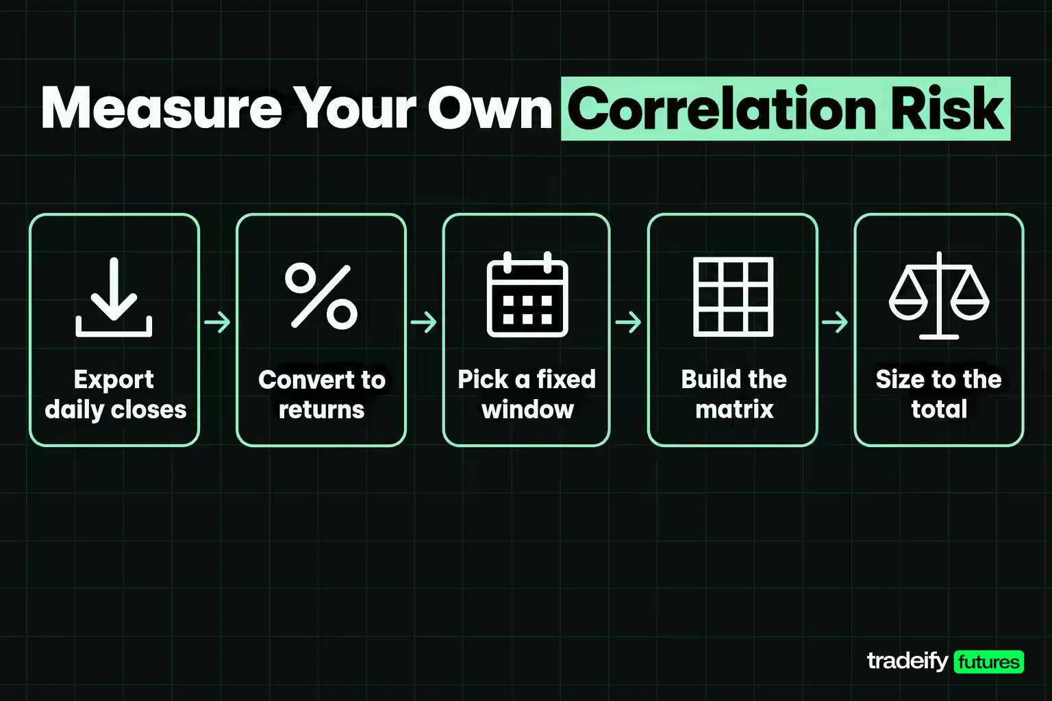
You do not need a risk system to measure correlation risk. A spreadsheet and your platform's daily closes are enough, and the whole routine takes a few minutes once the sheet is built.
- Export daily closes for every market you trade, for the same sessions, aligned by date. Drop any date that is missing in one market.
- Convert to returns. Use the percentage change (or log change) from one close to the next. Never correlate prices.
- Pick a window and keep it. Sixty sessions is a reasonable default. Twenty is noisy. Two hundred fifty is slow to react.
- Build the matrix. In Excel or Google Sheets, the CORREL function on two return columns gives one pair. Repeat for every pair you hold.
- Flip signs for shorts. If you are short one leg, multiply that pair's correlation by -1 before using it in the risk math.
- Compute combined risk. For equal-risk positions, use per-position risk × the square root of (N + 2 × the sum of the pairwise correlations). Compare that with per-position risk × the square root of N.
- Size to the total. If combined risk is above your limit, cut size across the book or drop the position that carries the most shared exposure.
- Recheck on a schedule. Recompute weekly, and also after any session where most of your positions moved the same way. Track each pair's 5th percentile, not just its latest value.
Two filters before adding any new position: does it share a driver with something you already hold, and would it stop out on the same session? If the answer to both is yes, you are adding size to an existing trade, not adding a new one. That is a legitimate decision, as long as you size it like one.
Related lesson: Concentration risk
Correlation Risk FAQ
What is correlated risk?
Correlated risk is exposure to several positions that tend to lose at the same time because they share a driver. A book of ES and NQ longs is one example. The risk is that losses arrive together, so the total loss on a bad session is closer to the sum of every position than the position count suggests.
What does a 0.95 correlation mean?
A 0.95 correlation means the two markets move together almost all the time, with about 90% of their daily variation shared. For risk purposes, two positions at 0.95 are close to one position. In this guide's 20-year study, ES and NQ ran at 0.92, and two positions at 1% each carried about 1.96% of combined risk instead of the 1.41% the shortcut gives.
Is higher or lower correlation better?
For positions in the same direction, lower correlation is better, because it reduces combined risk and spreads losses out. For a deliberate spread, long one market and short another, higher correlation is better because it keeps the trade a bet on the gap between them. A correlation that falls turns that spread into two directional trades.
What is an ideal correlation for a portfolio?
There is no single ideal number, so grade each pair rather than the whole portfolio. A pair whose rolling correlation stays above about 0.80 even at its 5th percentile, as ES and NQ did, should be treated as one position. A pair whose 5th percentile is near zero or negative, as ES and gold was, behaves like two positions at least some of the time.
Is 0.5 a strong correlation?
For position risk, 0.5 is stronger than it sounds. Only 25% of the variation is shared, but five positions at a 0.5 average correlation, each risking 1%, carry 3.87% of combined risk against the 2.24% the shortcut gives. Those five positions behave like 1.67 independent bets.
How often should you recalculate correlation?
Weekly is a sensible routine for a book of futures positions, plus a recheck after any session where most positions moved the same way. Correlations in this study shifted materially within months, so a number measured once and never updated can mislead you badly.
This guide is educational and describes a study of historical price data, not a recommendation to trade any instrument or strategy. Futures are leveraged, and losses can exceed what you expect when correlated positions move against you at once. Correlations measured on past data change without warning and do not predict future relationships. Results ignore commissions, slippage and margin. Evaluation and funded accounts are simulated, and results there may differ from live trading.


