



TL;DR: Quantitative trading means writing each trade decision as a rule and testing it on data before money is at risk. Three numbers decide whether a result is real, namely the break-even win rate, the trade count and the number of versions you tried. A 260-trade sample with a +0.096R mean has a t of 1.11, which is not yet evidence of an edge. Costs matter as much, since about $24 a round turn on one ES contract with a 5-point stop erases that whole mean.
Quantitative trading starts with a familiar problem. A setup wins seven of its last ten trades, and you have to decide whether that is an edge or a good week. Quantitative trading answers it by turning the idea into a rule precise enough to count, then letting data decide whether the rule deserves money.
It sounds technical, and parts of it are. The core is simpler. You stop judging a strategy by how the last few trades felt and start judging it by numbers you could hand to someone else.
This guide covers what quantitative trading is, where it came from, the main strategy families, the data and machine learning behind it, and how quant risk management works. It also works through one illustrative 260-trade sample to show the three numbers that separate a measured edge from a lucky stretch.
What Quantitative Trading Is
Quantitative trading is a method in which every trading decision (entry, exit, position size and when the system is switched off) is written as a rule that data can settle, tested on history, and then compared live against what the test predicted. The rule decides. The trader's job moves from picking trades to designing, measuring and maintaining rules.
Three activities get lumped together under this label, and they are worth separating.
- Quantitative trading is the measurement side: stating a rule in numbers and testing whether it has an edge.
- Algorithmic trading is the execution side: software sends the orders the rule calls for, without a human pressing buttons.
- High-frequency trading is a speed race in which firms compete in microseconds with co-located servers.
Most quant strategies end up automated, but a trader can run a quantitative method for months with a spreadsheet and manual orders. A simple test tells you whether you have one. Give your rule to another trader. If both of you would take the same trades on the same day, it is a rule. If you would not, part of the decision is still discretion.
Related lesson: Algorithmic trading
Quantitative vs qualitative analysis in trading
Quantitative analysis in trading uses measurable inputs (prices, volume, volatility, earnings figures, positioning data) and statistical tests to make decisions. Qualitative analysis judges things that resist measurement: management quality, the tone of a central bank statement, whether a chart "looks" strong.
| Question | Quantitative analysis | Qualitative analysis |
|---|---|---|
| Inputs | Prices, volume, volatility, reported data | Narrative, judgment, context |
| Decision | A rule fires or it does not | The analyst decides case by case |
| Testing | Can be backtested on history | Hard to test without hindsight |
| Main strength | Consistency and scale | Handles events with no history |
| Main weakness | Breaks when the market regime changes | Inconsistent and hard to audit |
The two are not enemies. Many quant firms use qualitative judgment to choose which ideas to test, and many discretionary traders use quantitative filters. The difference in quantitative trading is that the final trade decision belongs to the rule.
How Quantitative Trading Developed
Quantitative trading grew out of a handful of ideas that each made one more part of trading measurable.
- 1952, risk as a number. Harry Markowitz published "Portfolio Selection", which treated a portfolio as a tradeoff between expected return and variance. It later earned him a share of the 1990 economics Nobel.
- 1967 to 1969, probability applied to markets. Mathematician Edward Thorp, already known for card-counting research, co-wrote Beat the Market with Sheen Kassouf in 1967 and ran the hedge fund Princeton/Newport Partners from 1969 to 1989, built on hedging mispriced derivatives.
- 1978, the quant hedge fund. Jim Simons, who had chaired the Stony Brook math department, founded what became Renaissance Technologies in 1978. The Simons Foundation describes it as a hedge fund that pioneered quantitative trading.
- Mid-1980s, statistical arbitrage. A group at Morgan Stanley turned pairs trading into a systematic, many-position strategy, the start of modern stat arb.
- 2000s onward, speed and data. Electronic markets made high-frequency trading possible, and cheap computing put backtesting on every desktop.
The last step matters most for individual traders. The tools are now cheap. The discipline of measuring honestly is not, and that is where most of the work still is.
Quant Trading Strategies and What Each One Bets On
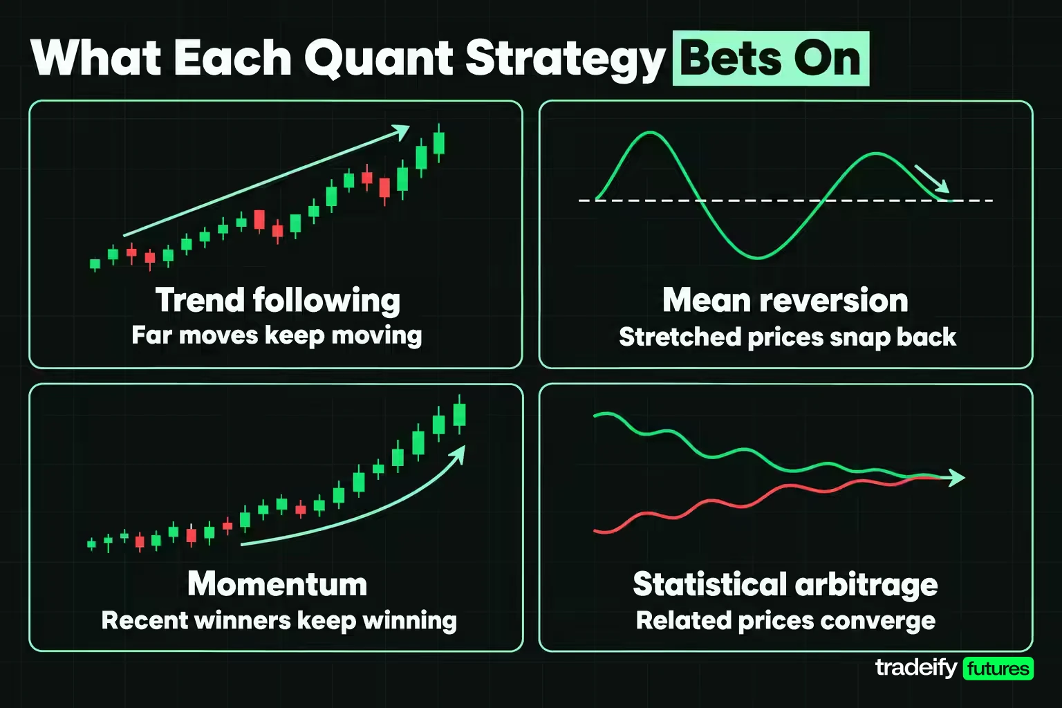
Every quant trading strategy is a bet on a specific market behavior repeating. Knowing which behavior a strategy bets on tells you when it should work and, more usefully, when it should fail.
| Strategy family | What it bets on | Typical failure |
|---|---|---|
| Trend following | Prices that move far keep moving | Choppy, range-bound markets cause repeated small losses |
| Mean reversion | Stretched prices snap back toward an average | A real trend keeps stretching and the stop takes a large loss |
| Momentum | Recent winners keep outperforming recent losers | Sharp reversals when crowded positions unwind |
| Statistical arbitrage | Related prices drift apart and then converge | The relationship breaks and the spread never returns |
| Market making | Earning the bid-ask spread on many small trades | Fast one-way moves leave the maker holding the losing side |
Trend following and mean reversion are opposite bets on the same chart, which is why they tend to win in different conditions. A trend system loses steadily in a quiet range and makes its year in a few big moves. A mean reversion system wins often and small, then occasionally takes the large loss that a breakout delivers. Neither is better in the abstract. The question is whether the payoff you measure matches the bet you think you are making.
Related lesson: Mean reversion trading
Statistical arbitrage in quant trading
Statistical arbitrage trades the relationship between prices rather than the direction of one price. The classic form is a pair: two instruments that usually move together, with the strategy buying the cheaper one and selling the richer one when the spread between them stretches. Index arbitrage applies the same logic to a futures contract and the basket of stocks it tracks.
Despite the name, it is not arbitrage in the risk-free sense. The bet is that a spread will converge, and sometimes it widens instead because the relationship itself has changed. That is why stat arb desks run many small positions at once and cut a pair when its behavior no longer fits the model.
High-frequency trading as a speed race
High-frequency trading uses very fast order generation, co-location next to exchange servers and direct data feeds to profit from tiny, short-lived price differences. In its 2010 Concept Release on Equity Market Structure, the SEC noted estimates that HFT typically exceeded 50% of total volume in US-listed equities, while also saying the term was not clearly defined.
Latency arbitrage is the clearest example. When the same instrument, or two tightly linked ones, trade on different venues, the faster firm sees a price change on one and trades on the other before the slower quote updates. The profit per trade is tiny, so the strategy only works at enormous volume and with the lowest possible latency, which is why HFT firms spend on co-location, microwave links and custom hardware.
For an individual trader, HFT is a race with no realistic entry. The edge is measured in microseconds and paid for with infrastructure. Quantitative trading at retail scale competes on a different axis: careful measurement, patience and rule discipline.
Where Quantitative Trading Is Used
Quantitative trading runs through far more of the market than hedge funds. Some of the most common applications:
- Hedge funds and CTAs. Systematic funds run trend following, stat arb and multi-factor models across futures, stocks and currencies.
- Market makers. Firms quote both sides of thousands of instruments and adjust prices with models of inventory risk and short-term order flow.
- Execution algorithms. Banks and asset managers split large orders with VWAP and TWAP algorithms so a big order does not move the price against itself.
- Index and ETF arbitrage. Traders keep futures, ETFs and their underlying baskets in line by trading the gaps.
- Risk desks. Quantitative models estimate how much a portfolio could lose and set limits before positions are opened.
- Individual traders. A single trader can backtest a written rule set on one futures contract, size it in fixed risk units and track whether live results match the test.
The individual case looks very different from the institutional one, but the logic is the same: a rule, a measurement, and a decision about whether the measurement is strong enough to trust.
Algorithmic Pattern Recognition in Quant Systems
Algorithmic pattern recognition sounds like software scanning charts for shapes. In practice, the hard part is not the scanning. It is defining the pattern so precisely that a computer and a human would flag the same bars. "A pullback in an uptrend" is an idea. "Price closes above its 50-bar average, then touches the 20-bar average without closing below it" is a rule.
A quant system is specified when four decisions are written in numbers. Most failed systems have two of them written and two left to judgment, which is enough for the backtest and the live account to disagree.
| Decision | What it must state | Example of a stated rule |
|---|---|---|
| Entry | The exact condition and the order type | Buy stop one tick above the signal bar high |
| Exit | Stop, target and time exit | 5-point stop, 2.5R target, flat by session close |
| Size | Risk per trade and how it converts to contracts | Fixed $250 risk, contracts = risk divided by stop value |
| Filter | When the system does not trade | No new entries in the 10 minutes around scheduled data |
The filter row is the one traders resist, because switching a system off feels like judgment. It is still a decision. If it is not written, the trade count, win rate and average return all describe a system that only traded the days you happened to approve.
Size deserves its own line because of contract rounding. On an E-mini S&P 500 (ES) contract, one index point is worth $50, so a 5-point stop risks $250 per contract. A $250 risk budget gives exactly 1 contract. A $125 budget with the same stop gives 0.5 contracts, and the system can only trade 0 or 1. Rounding up doubles the intended risk and rounding down skips trades, so the rule has to say which happens.
Related lesson: Position sizing
Data for Quantitative Trading
Data for quantitative trading falls into three groups: market data (prices, volume, order book), fundamental data (earnings, economic releases) and alternative data. The data is where most quietly wrong backtests go wrong, so the cleaning matters as much as the source.
Common data problems in quant research:
- Survivorship bias. Testing only on stocks that exist today leaves out the ones that failed, which flatters results.
- Look-ahead bias. Using a figure before it was actually published, such as a revised economic number or a daily close inside an intraday rule.
- Continuous futures contracts. Back-adjusted futures series splice contract months together. The adjustment changes historical price levels, so a rule based on round-number levels can break.
- Bar construction. A 5-minute bar from one data vendor may not match another's because of session times and late trades.
Sentiment and alternative data for quant models
Alternative data is anything outside the usual price and fundamental feeds: news and social media sentiment scores, web traffic, satellite images, credit card spending, shipping records. Institutional funds pay heavily for it because a signal nobody else has can last longer.
A free, well-documented example for futures traders is the CFTC Commitments of Traders report, which breaks down positioning by trader category. It reflects Tuesday positions and is generally published Friday at 3:30 PM Eastern, so a rule using it must not act on the data before Friday. That three-day lag is a simple look-ahead trap.
Sentiment data adds noise as easily as signal. Before trusting it, check how far back the history goes, whether the vendor revised past values, and whether the signal still works after costs.
Machine Learning in Quantitative Trading
Machine learning in quantitative trading uses algorithms (regression models, decision trees, gradient boosting, neural networks) to find patterns in data that a human would not write as a rule. The appeal is obvious. The risk is that financial data is short, noisy and changes behavior over time, which is close to the worst case for a flexible model.
A model with enough parameters can fit any history. The question is whether it learned something that repeats or just memorized the sample. Quant researchers guard against this in a few ways:
- Out-of-sample testing. Hold back a period the model never sees during training, and judge it only on that.
- Walk-forward testing. Train on one window, test on the next, then roll forward, so every test period comes after its training data.
- Time-aware cross-validation. Ordinary cross-validation shuffles data, which leaks future information into training. Financial cross-validation keeps time order and leaves gaps between training and test periods.
- Counting the trials. Every model variant, feature set and parameter tried is another chance to find noise.
That last point is backed by research. A 2014 paper in the Notices of the American Mathematical Society by Bailey, Borwein, Lopez de Prado and Zhu showed that with only five years of data, no more than 45 independent model configurations should be tried before a strategy with no skill starts to look like one with a Sharpe ratio of 1 in-sample. Machine learning makes it easy to try thousands.
Related lesson: Overfitting and look-ahead bias
Three Numbers That Test a Quantitative Trading Result
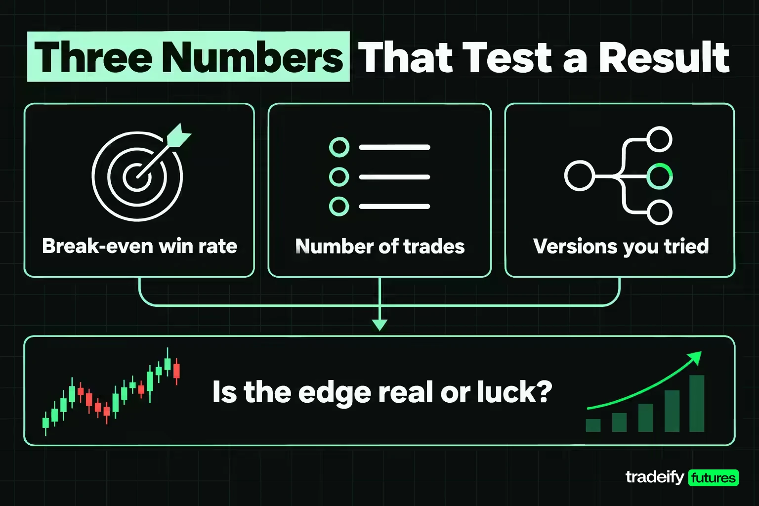
Three numbers decide whether a quantitative trading result means anything: the win rate the payoff requires, the number of trades the result needs, and the number of versions tried to find it. None of them needs code.
The break-even win rate your payoff requires
The break-even win rate is 1 divided by (1 + payoff ratio), where the payoff ratio is the average winner divided by the average loser.
| Payoff ratio | Break-even win rate |
|---|---|
| 1 to 1 | 50% |
| 1.5 to 1 | 40% |
| 1.8 to 1 | 35.7% |
| 2 to 1 | 33.3% |
| 3 to 1 | 25% |
This is also how to read a strategy someone is selling. A win rate means nothing without the payoff. A 60% win rate where winners are half the size of losers loses 0.1R per trade on average (0.6 x 0.5 minus 0.4 x 1), because that payoff needs 66.7% just to break even.
The number of trades the result needs
Take an illustrative 260-trade sample, built for this example rather than taken from a market. It has 104 winners and 156 losers, a 40% win rate.
| Group | Trades | Result per trade | Group total |
|---|---|---|---|
| Small winners | 34 | +0.5R | +17R |
| Medium winners | 30 | +1.5R | +45R |
| Target winners | 30 | +2.5R | +75R |
| Runners | 10 | +3.2R | +32R |
| Full stop losses | 132 | -1R | -132R |
| Early exits | 24 | -0.5R | -12R |
The average winner is +1.625R and the average loser -0.923R, a payoff of 1.76 to 1 and a break-even win rate of 36.2%. A 40% win rate clears that, and the sample nets +25R, a mean of +0.096R per trade. It looks like a working system.
Now measure the uncertainty. The per-trade standard deviation is 1.39R, so the standard error of the mean is 1.39 divided by the square root of 260, or 0.086R. The mean divided by its standard error gives t = 1.11, and the 95% interval runs from -0.073R to +0.265R. That interval includes zero. The two-sided p-value is about 0.27. Even the win rate is loose: its 95% interval runs from 34.2% to 46.1%, and the bottom of that range is below break-even.
So 260 trades cannot separate this system from one with no edge. That is uncomfortable, because a year of trading feels like plenty of evidence. It is one line in a much longer sample. The smallest mean this sample could detect with 80% power is 0.24R. Because t grows with the square root of the trade count, this same system needs 838 trades to reach t = 2 and 1,644 trades for 80% power, using the unrounded mean of 0.09615R and standard deviation of 1.3915R. At 260 trades a year, that is 6.3 years. These intervals assume trades are independent, which flatters a system whose trades cluster in the same conditions.
The number of versions you tried
Run 20 strategy versions with no edge at all on random data, and the best of them will still post a t of 1.87 on average. The chance that at least one clears the usual one-sided 5% bar of 1.645 is 64.1%. These figures come from a simulation of 200,000 sets of pure noise:
| Versions tried | Average best t from noise | Chance at least one clears 1.645 | Bar that keeps the family error at 5% |
|---|---|---|---|
| 1 | 0 | 5% | 1.96 |
| 7 | 1.35 | 30.1% | 2.69 |
| 20 | 1.87 | 64.1% | 3.02 |
| 45 | 2.21 | 90.0% | 3.26 |
| 1,000 | 3.24 | 100% | 4.06 |
A search produces a "discovery" whether or not the market contains one. The more versions you try, the better your best one looks, and none of that improvement is edge. Academic research reaches the same place. Harvey, Liu and Zhu (NBER Working Paper 20592) argued that after decades of data mining, a newly proposed return factor needs a t-ratio greater than 3.0, not 2.0, and that most claimed research findings in financial economics are likely false. For scale, an annualized Sharpe ratio of 1.0 over five years gives a t of only about 2.24, before any adjustment for how many variants were tried.
Related lesson: Trading expectancy
What Trading Costs Do to a Quant Backtest
Trading costs decide whether a thin quant edge survives. To see it, price the illustrative 260-trade sample on one E-mini S&P 500 (ES) contract. ES is worth $50 per index point, so a 5-point stop is $250 of risk, which is 1R. Every dollar of round-turn cost (commission, fees and slippage) is subtracted from every trade.
| Round-turn cost per contract | Cost in R | Net mean per trade |
|---|---|---|
| $2.50 | 0.01R | +0.086R |
| $5 | 0.02R | +0.076R |
| $12.50 | 0.05R | +0.046R |
| $25 | 0.10R | -0.004R |
The costs are illustrative, not a broker quote. The $12.50 row is worth a second look, because one ES tick is $12.50. A single tick of slippage on entry or exit costs as much as that whole row.
The break-even cost is 0.096R x $250, or $24.04 per contract per round turn. Above that, the sample loses money on every trade on average. A wider stop shrinks the cost in R terms: a 10-point stop risks $500, so $25 of cost becomes 0.05R instead of 0.10R. That is one reason short-term systems with tight stops are so sensitive to fills, and why the order type belongs inside the backtest rather than in a footnote.
Related lesson: Commission-adjusted futures breakeven
Quantitative Risk Management
Quantitative risk management sets the limits before the trade, in numbers, so the system's worst days are planned rather than discovered. A quant system can have a real edge and still fail if its risk rules do not survive a bad stretch.
The core tools:
- Fixed risk per trade. Express every trade in R, a fixed dollar risk, so results compare across instruments and stop sizes.
- Drawdown limits set in advance. Decide the peak-to-trough loss at which the system is cut or paused, and base it on the backtest's worst run plus a margin, because live drawdowns tend to exceed tested ones.
- Correlation limits. Two systems on ES and NQ are often one bet twice. Measure how their returns move together before adding both.
- Regime checks. A strategy built on quiet markets may break when volatility doubles. Track the conditions the backtest covered and flag when live markets leave them.
- Kill switches. Automated systems need a hard stop for runaway orders, data feed failures and repeated rejections.
Institutional desks add portfolio models such as value at risk, which estimates the loss a portfolio should not exceed on most days at a chosen confidence level. The weakness is the same one every model has: it is built on history and can understate the tail. That is why the simplest rule (never risk more on one trade than the system can lose many times in a row) still matters.
Related lesson: Risk of ruin
Pros and Cons of Quantitative Trading
Quantitative trading trades one set of problems for another. It removes a lot of emotional decision-making and adds the risk of trusting a model that has quietly stopped working.
| Pros of quantitative trading | Cons of quantitative trading |
|---|---|
| Rules apply the same way on every trade | A model built on history can break when the market changes |
| Ideas can be tested before money is at risk | Backtests are easy to overfit and hard to audit |
| Results can be measured and compared | Meaningful samples can take years to collect |
| Systems can scale across many markets | Data, software and execution costs add up |
| Removes in-the-moment fear and greed from entries | Overriding the system in a drawdown undoes the benefit |
The last row of the cons column is the one that catches individual traders. After four straight losses, skipping the fifth signal feels like risk control. In practice it means the live results describe a hybrid system nobody tested. If you override the rule, record it, so you can measure whether the overrides helped.
Related lesson: How to keep a trading journal
What a Quant Trader Does
A quant trader designs, tests, runs and monitors rule-based strategies. At a fund or trading firm, the work is usually split between three roles:
- Quant researcher. Forms hypotheses, tests them on data and writes up what survives. The work resembles scientific research more than trading.
- Quant trader. Runs strategies in the market, manages risk and execution, and watches for signs a model has stopped behaving as tested.
- Quant developer. Builds the data pipelines, backtesting systems and execution software that the others rely on.
The skill stack mixes statistics and probability, programming (Python is common for research, faster languages for execution), and an understanding of market structure: how orders fill, what moves spreads, how contracts roll. Most firms hire from mathematics, physics, computer science, engineering and finance, and graduate degrees are common for research roles.
For an individual, quantitative trading is a method rather than a career track. You do not need a PhD to write a rule, test it and track it. You do need the patience to collect enough trades and the honesty to count every version you tried.
Testing a Quantitative Trading Idea Step by Step
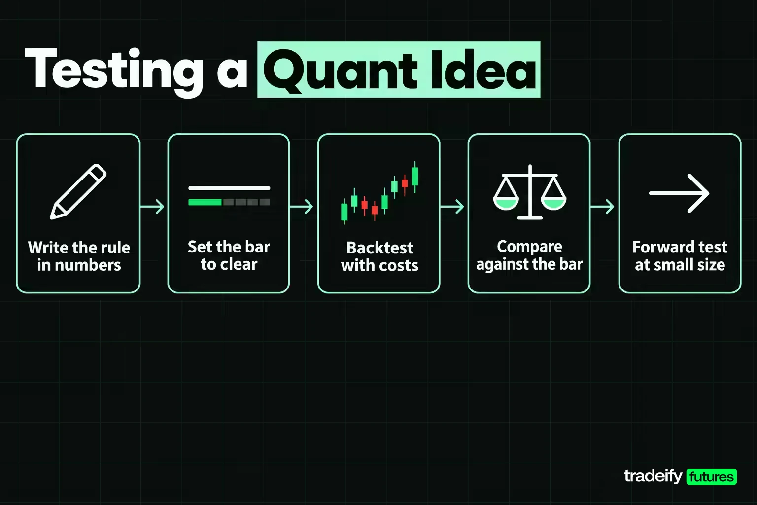
A quantitative trading research process does not produce strategies. It rejects the ones that never worked, which is most of the job. Run these steps in order:
- Write the four decisions (entry, exit, size, filter) in numbers and date the version.
- Decide how many versions you will test before you start, and log every one you run.
- Compute the break-even win rate from the payoff you expect, so the test has a bar to clear.
- Decide the smallest edge you care about, then work out the trade count needed to detect it.
- Run the backtest with costs and slippage in it, in R, at your real stop distance.
- Compare the result against the bar implied by your version count, not against zero.
- Forward test on new data at small size, and compare live results with the backtest's interval before adding size.
Step 7 is the only one that uses data the rule has never seen, so it is the one that most often changes the answer. If the live mean lands outside the tested interval, the rule goes back to research rather than getting more size.
Tracking quant test results and versions
Two records make the steps for testing a quantitative trading idea auditable later: the statistics for each test, and a log of every version tried.
Running a quant system on a funded account
A quant system built for a funded account has to fit that account's rules before it is tested. On our accounts, automated strategies follow a few rules. An algorithm is allowed only if you own the strategy exclusively, it is not shared, and it is not high-frequency trading. Tradovate API access is limited to live funded accounts. All positions must be closed by 4:45 PM ET, so a system that holds overnight would need redesigning to trade on our funded accounts, which are simulated.
Related lesson: Forward testing and walk-forward analysis
Quantitative Trading FAQ
What is quantitative trading?
Quantitative trading is trading in which entry, exit, size and filter decisions are written as rules and tested on data before money is at risk. The rules are then executed consistently, by software or by hand, and live results are compared against the test.
What is quantitative analysis in trading and how is it used?
Quantitative analysis in trading uses measurable data and statistics to evaluate markets and strategies. Traders use it to define signals, test rules on history, size positions in fixed risk units and decide whether a result is strong enough to trust.
What is the 7% rule in trading?
The 7% rule is a stock-investing guideline popularized by Investor's Business Daily: sell a stock if it falls 7% to 8% below what you paid for it. IBD suggests a tighter 3% to 5% in weak markets. It is a loss-cutting rule for stock buyers, not a futures rule, and a quant system would test any such stop rather than adopt it on authority.
Who is the most famous quant trader?
Jim Simons is the name most often given. A mathematician who chaired the Stony Brook math department, he founded what became Renaissance Technologies in 1978, a firm the Simons Foundation describes as having pioneered quantitative trading. Edward Thorp is another early figure, known for applying probability to markets from the late 1960s.
What is the difference between quantitative trading and algorithmic trading?
Quantitative trading is the research and measurement: stating a rule and testing whether it has an edge. Algorithmic trading is the execution: software placing the orders the rule calls for. Most quant strategies end up automated, but the two are separate skills.
Is quantitative trading profitable?
Not by default, because quantitative describes the process and the process mostly rejects ideas. Its main value is showing you early, in numbers, when a strategy is not working.
Futures and leveraged trading carry substantial risk, losses can exceed what you expect when a model meets conditions it was not tested on, and the sample, costs and simulations in this article are illustrative arithmetic, not market results. Funded and evaluation accounts are simulated, and nothing here is investment advice or a recommendation to trade any instrument.


